The problem: Infrared emission of glass |
  
|
The problem: Infrared emission of glass |
|
This example shows how a three layer coating on glass is designed for a certain application. The application of the layer system under discussion is to reduce the infrared emission of architectural glass used in office buildings or private houses. In addition to this purpose you can use the coating also for achieving a certain appearance, i.e. a certain color of the pane.
In a first step we identify the problem of infrared emission by inspecting the performance of uncoated glass.
Start CODE and activate File|New to start with an empty configuration. Then press F7 to enter the treeview level. For our considerations we need optical constants of glass from the infrared to the near UV. The data that come with this tutorial contain a fixed data set that you can use. Create in the list of materials a new object of type 'Imported dielectric function'. Open it and load with the local command File|Open the file glass.df. Press the 'a' key to autoscale the graphics and you should find this:

To compute the emission of a glass pane with these optical constants define a layer of type 'Thick layer' with a thickness of 4 mm between two vacuum halfspaces.
Glass is a material with a quite large infrared absorption. In the spectrum list, define two spectrum simulation objects and use them to compute the infrared reflectance and transmittance spectrum (50 ... 5000 1/cm, 500 data points) of the pane (assume normal incidence of light). Call them 'R IR' and 'T IR'. When you are ready use the main menu command Actions|Create view of spectra to generate a simple view showing the 2 spectra. The configuration tu1_ex1_step0.wcd contains the configuration that you should have by now:
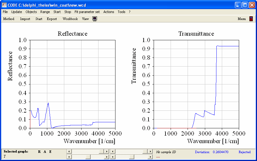
The transmittance is zero, at least below 2200 1/cm. Due to the rather low reflectance and the vanishing transmittance such a window has a quite large infrared emissivity. If it is used as the inner pane in a double glass window it has room temperature (i.e. 300 K) and acts as an infrared radiation source which leads to large radiation losses.
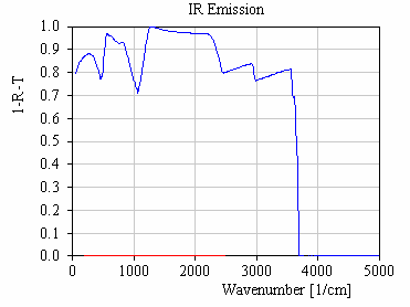
With CODE you can compute these losses the following way. Create a new spectrum object of type 'R,T,ATR' and compute the emissivity by setting the spectrum type to 1-R-T. You should get this spectrum:
To compute the emitted power per area this spectrum has to be multiplied by the spectral distribution of a black body at 300 K (Planck radiation formula), followed by an integration over all frequencies. You can do these muliplication/integration steps applying a spectrum product object. This can be created in the list of integral quantities. Create such an item, and open with Edit the corresponding window where you have to define the black body emission. First you are asked for a nickname. Call the quantity 'Emitted power' as shown below:

Now you have to specify the unit:
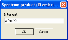
Now you have to enter a scaling factor (use 1 here) and the number of decimal places for the number output (use 4). Now the following window opens where you have to define the spectral distribution of the blackbody radiation:

What formula do you have to type in? Here comes a short repetition of one of your physics courses. The formula to be used for the blackbody emission is developed and checked in the following. The Planck radiation formula giving the energy density per frequency interval in a cavity is
Here we have switched to wavenumbers for later convenience.
Assuming that the energy moves with the speed of light distributed equally into all directions one can compute the energy per time that passes a small leak in the cavity to the outside. The energy density per solid angle is then ![]() .
.
To obtain the energy per time and area crossing the leak we have to compute the integration over all those contributions with a speed component into the outside:
Inserting what was found for the energy density gives
which is what we need to compute the total emission of the absorber.
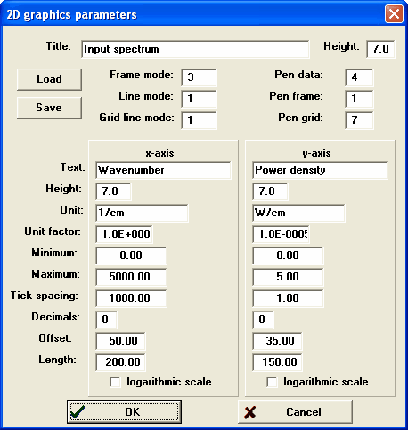
Now you can go back to the spectrum product object and type in the formula 3.74*10^(-12)*X^3/(EXP(1.439*X/300)-1). Note that T was replaced by 300 K (room temperature). Set the range of the object to 50 ... 5000 1/cm with 200 data points. Then press Go! to compute the spectral distribution of the emitted power of a blackbody at 300 K. Here it is:

The graph has been drawn with the following graphics parameters:
To compute the emitted power per area you now have to assign the simulated 1-R-T spectrum to the spectrum product object. Place the cursor in the spectrum column of the list of integral quantities and hit the F4 key several times. This way you move through all spectra in the spectra list. Stop at the IR emission spectrum. Then go to the next column (sim/exp) and select 'Simulation' (also by pressing the F4 key several times). Now select the Update menu command in the list of integral quantities:
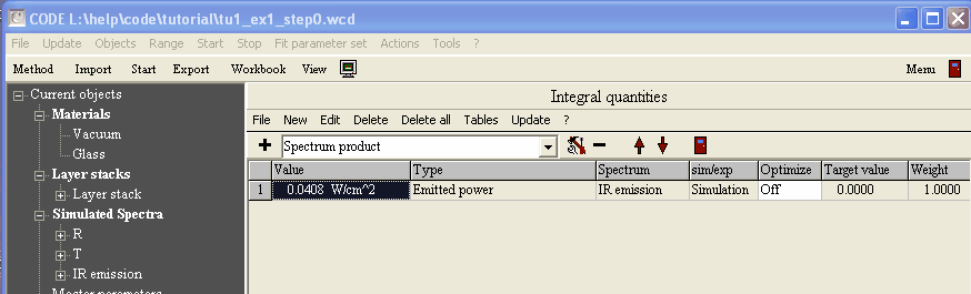
One gets a value of 0.0408 W/cm2. This means that we have 408 W losses by infrared emission of the pane per square meter!
Is that right? There is simple way to check this value by comparison to the emission of a perfect blackbody radiator which is given by the Stefan-Boltzmann law:
![]()
Here one gets 460 W/m2 which is a little higher because the emissivity of the glass is lower than 1.
The program configuration obtained up to now is saved as tu1_ex1_step1.wcd in the data folder of this tutorial.