Navigation:  Working with the workbook > Generating graphs with the workbook

In many cases it is convenient to visualize workbook data in graphs in order to inspect relations intuitively. This section shows how you can do that with the built-in Collect object.

The Collect object is able to display spectra (or other data which are series of x-y-data pairs) in 2D and 3D graphs. In the following I refer to the individual items as 'spectrum'. The spectra to be displayed are collected in a list where parameters like pen color or line style can be set for each spectrum. Working with Collect as a stand-alone program, you can transfer spectra from SCOUT or CODE to Collect by drag&drop. Of course, you can also import spectra from data files.

 

Copying data from the workbook to Collect

In order to display workbook data with the Collect object they must be copied into its list of spectra. This copy process can be initiated using several workbook commands, following always the same scheme:

•Select the workbook sheet from which you want to copy

•Select the cell where the copy process should start

•If you want to generate a new graph clear the Collect spectra list with the command Graph|Clear graphics window. If you do not clear the data the following copy action will add the new data to the ones that are already present in Collect.

•Activate the appropriate copy command in the Graph submenu

•Switch to the Collect object to set the graphics parameters that control the graph

 

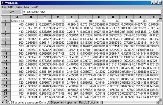
To explain the different copy commands the data created in the parameter variation example are used:

 

 

These copy commands can be used:

 

Graph|x,y downwards

This command is used to copy just a single spectrum starting at the selected cell. Placing the cursor in the cell A2 SCOUT will start reading the first x-value in that cell (400), then go to the cell B2 to the right of it and read the first y-value (-0.996312). Then it will inspect the cell A3. If it isn't empty the next pair of x- and y-values is taken from the cells A3 and B3. Afterwards cell A4 is tested for being empty, and so on. The reading process finishes when the first empty cell in column A occurs.

The collection of the found x-y-pairs is then treated as if it had been imported from a data file: SCOUT generates an equidistant set of x-values covering the same range of x as the input data. The corresponding set of y-values is obtained by linear interpolation from the original x-y-pairs. If, like in this example, the x-values are equidistant already, no changes to the spectrum occur. Finally the equidistant set of data is sent to the Collect spectrum list.

With appropriate graphics settings one would get from the sample data a graph like this:

Graph|x,y1, y2, ... downwards

After this command SCOUT starts at the cursor position and reads x-values downwards until an empty cell is found. Starting at the initial cursor position, it reads y-values moving to the right until an empty cell is found. If there are n rows of x-values and m columns of y-values the program expects the array of n*m cells to be filled with numerical data. It will pass to the Collect window m spectra being all defined on a grid of n spectral points.

Starting the copy process at cell A2 one could arrive here:

 

Obviously, the names of the individual spectra are not set automatically. You would have to do this manually which can be tedious if you have many spectra. If each spectrum is characterized by a number you can use the next command to achieve a reasonable automatic assignment.

 

Graph|_, p1, p2, ..., x,y1, y2, ... downwards

After this command SCOUT starts at the cursor position and inspects the cells to the right until an empty cell is found. If there are m non-empty cells the entries of these cells are expected to be numerical values which are used as parameter value for the spectra. Starting in the cell directly below the selected cell SCOUT proceeds as described above, i.e. it reads n x-values downwards and m spectra to the right. The spectra and the corresponding parameter values are passed to the Collect window where the display can now be more complete since each spectrum has its own 'name' given by the parameter value.

Starting at cell A1 in the example data shown above, one can achieve the following chart:

If, like in this case, each spectrum has a different parameter, and the list of spectra in the Collector window is sorted (which is done automatically for you if you apply the command Graph|_, p1, p2, ..., x,y1, y2, ... downwards) you can click on the buttons promising 3D plots. You get (after some plot parameter adjustments):

or

 

Graph|x,y from left to right

This command works like Graph|x,y downwards. The difference is that now the x-values are read from left to right, starting at the selected workbook cell. Below each x-value SCOUT expects a valid y-value.

Selecting cell B1 in the sample data, and applying this command one gets a plot of cos(delta) at 400 nm vs. SiOx layer thickness:

 

Graph|x,y1, y2, ... from left to right

This command is used to read many spectra from left to right, like the 'downwards version' discussed above. Note, however, that you should avoid to import too many data sets. A number larger than 40 is not supported by SCOUT.

 

Graph|_, p1, p2, ..., x,y1, y2, ... from left to right

This is the 'left to right' version of the similar downwards command described above. Once more, make sure that there are not too many rows to process. SCOUT will not work properly for more than 40 rows.

For sample data restricted to 21 spectral points in the range 400 ... 800 nm as shown here

 

 

one gets the following picture (starting with cell A1 selected initially):

 

Plots with well-defined and different parameters for each data set can also be done in 3D:

 

 

Displaying the data in the Collect window

Once the data are copied by one of the commands above the Collect window is opened:

 

 

The indiviual spectra are collected in a list which is opened by the Show List command:

 

 

Each spectrum has a parameter, a color, a line type, a name and a spectral unit.