Navigation:  Example 1: Low-E coatings > Visible appearance of Ag-coated glass

Now we are going to investigate how the Ag-coated window performs in the visible spectral range. In the spectra list, create two more spectra and name them 'R Vis' and 'T Vis', respectively. Set the spectral range for both spectra to 300 ... 800 nm with 100 data points. Press Recalc and adjust the graphics parameters to get the following graphs:

 

 

 

 

It is now time to setup a convenient main view. Expand the treeview branch Views and right-click the subbranch 'Spectrum view'. We will generate the following view items:

 

•Drag the new spectra 'R Vis' and 'T Vis' to the list of view items like it was explained in the 'Quick start ...' section of the SCOUT technical manual.

•In the dropdown box of the view item list, select the new type 'Rectangle' and generate a new object of this type.

•Drag the object 'Layer stack' to the view item list and drop it there. This will display the layer stack graphically.

•Drag the integral quantity 'Spectrum product' (the one that we called 'Emitted power') to the list of view items. This will show this quantity in the view.

 

Now press F7 to inspect the main view:

 

 

Obviously we have to do some re-arrangements of the view elements. Remember that each view element is a rectangle which can be moved and re-sized with the mouse in the main view (see the section about views in the SCOUT technical manual). Try to get the following main view appearance:

 

 

The corresponding view element list looks like this:

 

 

The color of the rectangle in the center of the view has been changed to gray.

 

Back to optics: To visualize the influence of the Ag layer, select the Ag layer thickness as a fitting parameter. Set the range of the fit parameter to 0 ... 20 and create a slider:

 

 

With the slider motion you can now test values between 0 and 20 nm Ag layer thickness. Watch the changes in the spectra while 'moving the thickness':

 

 

You may notice that you can reduce the emission from 408 to 61 W/cm^2 with a silver thickness of 2.5 nm only. The spectra in the visible are hardly influenced by this thin metal film. However, it is not possible up to now to produce large scale Ag films with that thickness because Ag starts to grow as an inhomogeneous island film on glass. These island films are very colorful and do not help to reduce infrared emission very much (see SCOUT tutorial 2). You must have a thickness of 7 to 8 nm to produce a homogeneous film with the wanted properties. These thicker films reduce the transmission of the window significantly and are also not neutral in color.

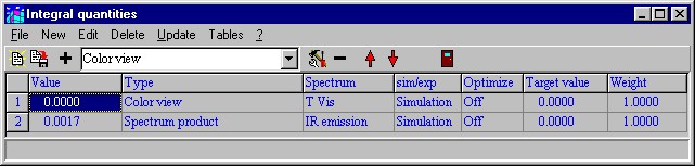
To directly visualize the color, open the list of integral quantities and create an object of type 'Color view'. As with the spectrum product object, assign the simulated transmission spectrum to the 'Colorview' object:

 

 

Drag the new integral quantity from the treeview to the list of view items and drop it there. This will generate a view object that can display the color view object in the main view. Move the new view element to the bottom of the center rectangle and size it the following way:

 

 

The program configuration obtained up to now is saved as tu1_ex1_step3.wcd in the data folder of this tutorial.