Navigation:  Parameter fitting > Automatic fitting

After you have found reasonable start values for the fit parameters by manual or visual variation you can activate the automatic fit by Start in the main window. The automatic parameter variation uses the methods described below to optimize the fit parameters, i.e. to minimize the deviation. Whenever the model improves you'll get an update of the status bar at the bottom of the main window. If you have defined a view in the main window it will be re-drawn based on the improved model. In addition, all open dielectric function and spectrum windows are updated to keep you informed about the progress of the model.

With Stop you stop the fit activity. It is also possible that the fit algorithm automatically decides to stop the fit. This occurs if there seems to be no progress any more.

 

Alternatively to the Start and Stop menu commands you can use the Start button in the toolbar. This must be used if the menu has been hidden. After the fit has been started the button turns into a Stop button which can be used for manually stopping the fit activity.

 

Pre-fit parameters

The mechanism of a quick pre-fit has been introduced with object generation 3.90. You can define several sets of parameters (called pre-fit sets) which are tried before the actual automatic fitting is started. The parameter values of the best fitting pre-fit set are then used as starting values for the automatic fit.

Pre-fit sets are created and selected using 4 buttons with red labels on the panel above the fit parameter grid:

 

 

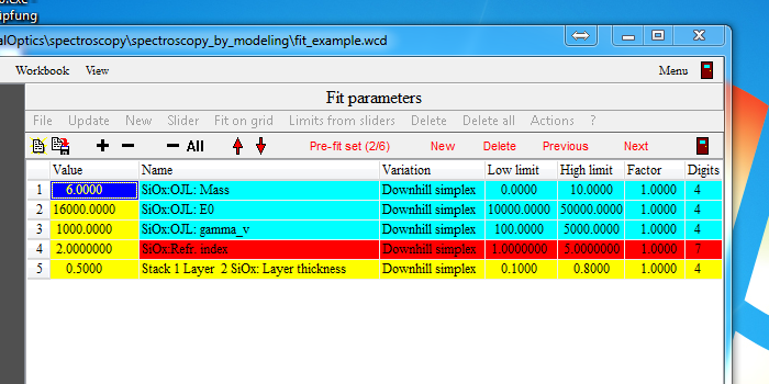
'New' takes the current fit parameter values and stores them as additional pre-fit set.

'Delete' deletes the selected pre-fit set (which is indicated by the label 'Pre-fit set (2/6)')

'Previous' selects the previous set. If the current set is the first, the last set is selected.

'Next' selects the next set. If the current set is the last, the first set is loaded.

 

Pre-fit sets are stored in configuration files.

Pre-fit sets are also stored in fit parameter set files.

 

 

List of fit parameter sets

Quite advanced fitting algorithms are possible using a sequence of fit parameter sets. These can be defined in the list of fit parameters sets which is opened by right-clicking the wanted element in the treeview branch Fit parameters sets in the main window. A list may look like this:

 

 

Each fit parameter set has a user-defined Name to characterize it, a Time threshold (specified in seconds), a Deviation threshold, and a Tolerance threshold. The file containing the fit parameter set must be given by Filename. All fit parameter set files must be stored in the directory where the loaded SCOUT configuration file is located. Fit parameter set files are created using the Fit parameter set|Store commmand in the main window (see above).

SCOUT loads each set in the list and fits until the user-defined time threshold or the user-defined deviation threshold is reached. The third quantity that determines the termination of the automatic fitting is the tolerance which is an internal quantity of the downhill simplex method used to optimize the parameters (see below).

Then the next fit parameter set is loaded until the end of the list is reached.

 

Downhill simplex method

The automatic parameter fit for each fit parameter set is done by a routine that makes use of the so-called downhill simplex algorithm. This method is a simple, but stable algorithm to minimize a function (the fit deviation) that depends on many parameters. See [Press 1992] for a detailed description.

In almost all cases this method will find the next local minimum of the fit deviation. There is no guarantee, that this is the global minimum as well. It is the responsibility of the SCOUT user, i.e. you, to select good starting values close to the global minimum, or at least to inspect the final SCOUT solution carefully. In many cases you can   achieve a very good fit performance by finding the right sequence of fit parameter sets and making use of 'fit on a grid' steps.

 

Automatic processing of many samples: Batch fit

In cases where an automatic fitting scheme is found, you can apply it to a sequence of input spectra. This SCOUT feature is described below.