Navigation:  Special computations > Parameter variation

Objects of this type perform the variation of a single parameter of the optical model and compute a series of points with x- and y-coordinates which are computed according to user-defined expressions. The dialog for the object settings is this:

 

 

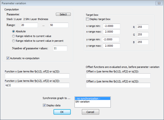
You can define an absolute range for the parameter variation, or a range relative to the current values (like +/- 5 nm for a thickness) or a variation in percent with respect to the current parameter value (like +/- 2%). If you use relative variations you should take an odd number of points and do the variation symmetric around the current value.

 

The functions for the x- and y-value computation are very general expressions: You can use the usual mathematical symbols and/or refer to the fit parameters (fp(4) returns the value of the 4th fitparameter), optical functions (of(2) gives the value of the 2nd optical function) and integral quantities (iq(6) delivers the value of integral quantity number 6).If you leave out the definition of "Function x" as shown in the screenshot above, the parameter values of the variation are taken as x-values. The given example shows how the first integral quantity depends on the SiN thickness.

 

In some cases it turned out to be advantageous to compute an offset for the x- and y-values, e.g. to perform a small color correction. You can do so by setting expressions for the functions "Offset x" and "Offset y" to the right.

 

In case you want to overlay several parameter variation results in one view you can synchronize the graphics settings (see below) to a given "master" object.

 

Once the settings dialog is closed a graphics dialog opens which is used to set 2D graphics for the presentation of results in a view. In order to show a special computation object you have to drag-and-drop it to a list of view elements.

 

The given example leads to this main view appearance:

 

 

 

Special computation objects compute the position of the minimum and maximum y-values. You can extract these numbers as optical functions, specifying the name of the object and using the arguments minimum_x, minimum_y, maximum_x and maximum_y. Optical functions can be viewed in views through drag-and-drop as well.

The example above uses the following optical functions:

 

•SiN variation(minimum_y)

•SiN variation(minimum_x)

•SiN variation(maximum_y)

•SiN variation(maximum_x)