Since many people asked for a convenient description of scattering losses due to interface roughness we have developed a special layer type which may help in many cases.

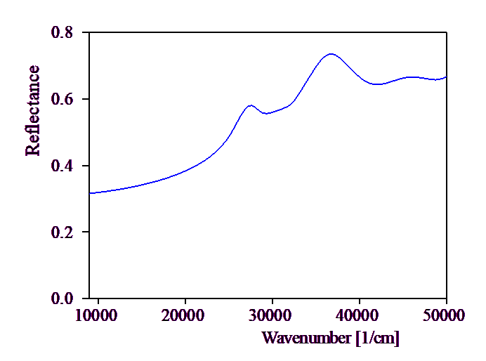
To demonstrate the application of this feature we consider a simple interface between vacuum and silicon in the Vis/UV region. The reflectance (10° angle of incidence) is the following:

To introduce roughness losses a layer of the new type 'Rough interface' is inserted between the vacuum and the silicon halfspace:

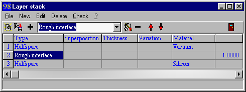
To get access to all the layer parameters you have to expand the window a little:

The most important parameter is given in the 8th column ('1.0' is the default). Here you can define a function which determines a frequency-dependent correction factor which multiplies both the amplitude reflection and transmission coefficient of the interface. Click on the '1.0' and type a 0.5 instead. Now you have (after a re-calculation) the following spectrum:

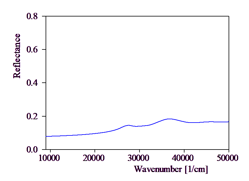
The amplitude reflection coefficients are multiplied by 0.5 which means that the intensity is now one fourth only.

Of course, you may want to define a frequency dependent correction since scattering losses typically are more pronounced for small wavelength than for large ones. You can do so. The wavenumber can be introduced into the formula as the variable 'X' as shown below:

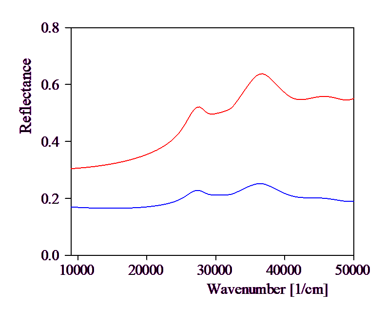
Now for low frequencies the correction factor is close to one and for high frequencies it gets larger:

Here the blue curve is the new spectrum including scattering losses whereas the red one shows the original spectrum without interface roughness for comparison.

As you can see you can be quite creative and implement all kinds of scattering loss corrections specifying the corresponding 'loss function'.

In order to increase your flexibility even more the 6th and 7th column of an interface roughness layer specify two possible fit parameters that you can use in the formula. As shown in the following example you can refer to the two parameters as C1 and C2, respectively:

Of course, the given formula gives the same correction factor as before, but now you could fit the C1 and C2 values to experimental data.

Here is an example: setting C1=0.8 and C2=100000 and loading the previous spectrum (that was created using the explicit formula 1/(1+X/500000) ) as a 'measured spectrum' the following situation is created:

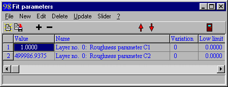
Declare the two roughness parameters as fit parameters and start the downhill method. After a short while the original values are recovered by the fit:

We hope that this explanation of the interface roughness layer type is clear enough and that two adjustable parameters in a scattering loss model turn out to be sufficient.

Current limitations

•interface roughness layers cannot be used in connection with anisotropic layers.

A 'real world' application example of a roughness correction is discussed in [Valk 1998A].