We can now prepare the parameter fit. Please follow exactly the next steps.
1. Open the fitting module with the menu command Tools|Optimize:
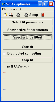
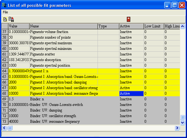
2. Push the button 'Select fit parameters'. This will open a list which will show all possible fit parameters. Move down the list until the cursor reaches item 67. Move the cursor to the column 'Active' and change the value by pressing the F4 key. Stop when the state of parameter 67 is 'Active'.
3. Move to line 68 and set the resonance frequency parameter to 'Active' as well.
All other parameters should be set to 'Inactive'.
4. Close the list. Another window should popup (if not, push the button 'Show active fit parameters'). This is a list which displays the parameters that are varied in the fit:
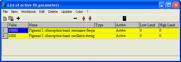
Keep this window open in order to watch the changes of the fit parameters during the optimization.
5. Now press the 'Spectra' button in the SPRAY optimizer window. This opens a list of spectra that are used to define the target of the fit:
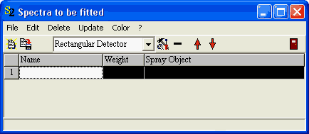
Up to now, you can only use spectra computed by 'Rectangular detector' objects in SPRAY for a comparison to measured spectra. In order to fit the spectrum of a rectangular detector just drag it from the list of geometric objects in SPRAY to the list 'Spectra to be fitted'. In our case, the window looks like this after drag&drop of the detector object:
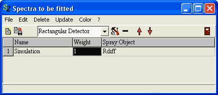
6. Use the Edit command to open the spectrum window. With the Range command you have to select the spectral range for the comparison of measured and simulated spectra:
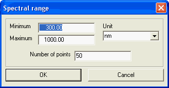
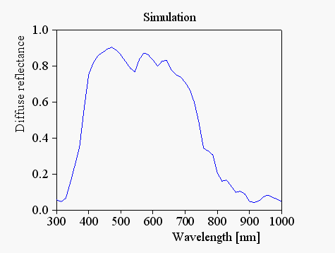
With the command Receive data you can transfer the current simulated spectrum of the SPRAY detector object to the spectrum which is used for optimization:
7. Now use the Experiment command to open the subwindow which is used to import a measured spectrum. In this window, use the Import command and load the spectrum from the file measured_spectrum.std (standard file format):

8. Close the window with the experimental spectrum, and verify that the spectrum window now shows both the simulated and the measured spectrum:
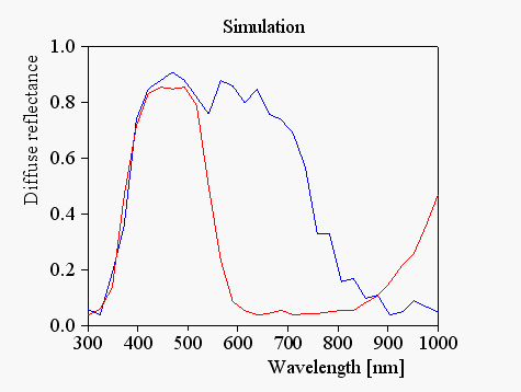
The configuration work is done now and we can proceed to the final fit action.