The first thing you should do is to define optical constants for all materials relevant for the given problem. You have to do that in the list of materials which is an important part of every SCOUT configuration. Objects in SCOUT are managed in several lists which are all branches in the so-called object treeview. In order to modify SCOUT lists or objects you must select them in the treeview and then do your changes.

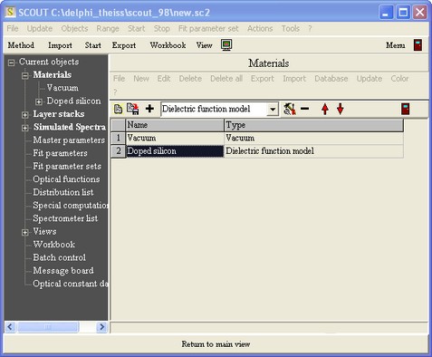
To get access to all SCOUT objects we have to switch from the main view (that we have seen up to now) to the treeview level by pressing F7 on your keyboard (Pressing F7 again leads you back to the main view). The treeview level looks like this:

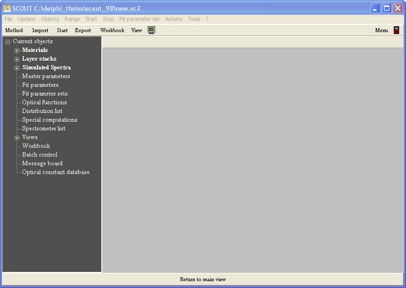
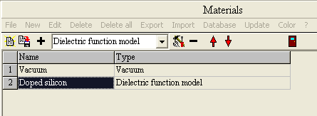
Display this list of materials by a right mouse click on the treeview branch Materials:

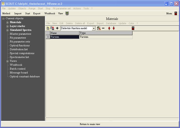
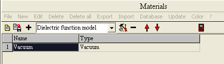
In the following we will work in the list of materials, i.e. in the right part of the SCOUT window. Note that this is a subwindow with its own menu and buttons:

In our case we need vacuum and doped silicon only. Vacuum is already defined, so we just have to define an optical constant model for silicon. The term 'optical constants' is often used for both the so-called dielectric function as well as its square root, the complex refractive index. Press the speed button labeled as '+' to create a new dielectric function of type 'Dielectric function model'. The + button or the New command in a SCOUT list always generate a new object of the type currently selected in the dropdown box to the right of the + button. Now the list is a little longer:

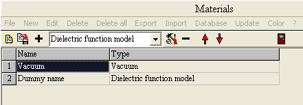
Place the cursor to the name 'Dummy name' as shown above and start to type 'Doped silicon'. Hit the return key when you are finished. The list should be this now:

Now we have to setup the dielectric function model for the new material called 'Doped silicon'. Note that the treebranch Materials has now a new branch called 'Doped silicon' which you can open by clicking on the little + to the left of Materials:

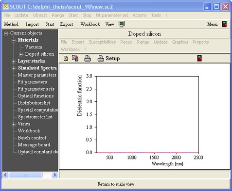
Right-click the treeview branch 'Doped silicon'. The list of materials disappears and the new object 'Doped silicon' is shown:

First we define the spectral range that we are going to investigate in the following. The Range command of the 'Doped silicon' menu (underneath the title 'Doped silicon') opens the corresponding dialog where you should define a spectral range from 100 to 3000 1/cm using 100 data points. The dialog should look like this:

Now we define the dielectric function model by creating two susceptibilities in the so-called susceptibility list. Open this list by clicking the + to the left of the 'Doped silicon' branch of the treeview. The right-click the branch 'Susceptibilities':

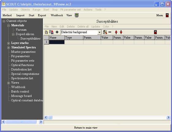
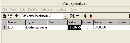
Create a constant background susceptibility by pressing the '+' button to the left of the dropdown box which shows the new object type 'Dielectric background'. Change its name to DB (select the name column, type in DB and press Return). Set the real part of this susceptibility to 11.7 (which is a good number for silicon, just believe it) such that the susceptibility list appears as follows:

If you have problems changing values in such lists please consult the section 'List properties' in the 'Technical notes' section of the SCOUT help.

Secondly you have to add a Drude susceptibility which will describe the response of the free charge carriers. Select the susceptibility type 'Drude model' in the dropdown list and create with '+' a new Drude term. Change the name of the new susceptibility to 'Carriers' but leave the default values of the Drude parameters unchanged:

Now right-click the 'Doped silicon' treeview branch. This closes the susceptibility list and re-opens the graph that shows the dielectric function. Click on the menu command Recalc  to compute the dielectric function based on the two susceptibility terms that you have defined. The graph should now look like this:

We are seeing only part of the data. Press the 'a' key on the keyboard (which abbreviates 'Autoscale') and see that the full range of the data:

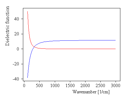
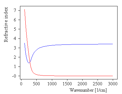
The red curve shows the imaginary part, the blue one the real part of your dielectric function model. If you prefer to see the complex refractive index apply the menu command Property|Refractive index. SCOUT will now display the refractive index (real part in blue, imaginary part in red) and do an automatic scaling:

This is a suitable moment to mention that the document 'Graphics course' delivered with SCOUT shows you how to master the program's graphics features. This is not repeated here, but it would be very helpful if you could handle at least the basic mechanisms to move around in your SCOUT graphs.

Now the optical constant model for doped silicon is complete. It is advisable to save your work from time to time. The most convenient way to do this is to save the complete program configuration in a binary SCOUT configuration file. This can be done by the command File|Save As in the main window. You can reload a SCOUT configuration file with File|Open any time and continue your work.