Navigation:  Example 1: Effective medium tutorial > Step 2: Testing simple effective medium models

Now, since we are convinced that a homogeneous silver layer is not the right choice, we have to do something else. Knowing that we have an inhomogeneous silver-vacuum mixture, we could try some simple averaging formulas that can be found in literature. This section shows how to do that. In the end, however, we will find that all the simple approaches are not flexible enough to lead to a good description of the experimental spectra.

 

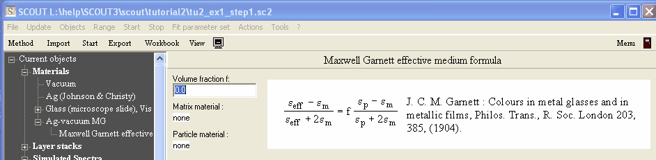
Maxwell Garnett formula

This effective medium approach was developed for very diluted collections of small particles (in dipole approximation). It contains one resonance, namely the dipole resonance, which occurs in the case of low volume fractions if the real part of the silver dielectric function is equal to -2. For higher volume fractions the resonance shifts to smaller frequencies due to electric interactions of the particles. The volume fraction is the only parameter that is used to describe the geometry of the inhomogeneous system.

In the Bergman representation the Maxwell Garnett formula has the following spectral density:

 

 

There is just one δ-function (representing the dipole resonance mentioned above) which moves from n=1/3 at f=0 to n=0 at f=1.

 

Here are the basic steps that you have to do for all effective medium models in SCOUT. Open thematerial list (which by now contains vacuum, silver and glass). Create a new object of type 'Maxwell Garnett model' and call it 'Ag-vacuum MG'. In the treeview this object will have a subbranch called 'Maxwell Garnett effecitve medium formula'. With a right-click on this branch you open the following window:

 

 

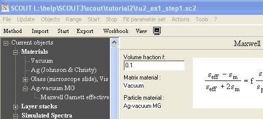
Three things have to be done: Enter a first guess for the volume fraction, e.g. 0.1, and specify the matrix material and the embedded particle material. The material objects must be dragged from the treeview to the white rectangles which are now still labeled as 'none'. The drag operation can be done the same way as you have already practised in tutorial 1 for the assignment of materials to layers. Push down the left mouse button at the treeview item representing the wanted material. Then move the cursor (while holding the mouse button down) to the white 'landing zone' and release the mouse button. Do that for vacuum as matrix material and silver as embedded particle material:

 

 

 

Now you can open the effective medium object 'Ag-vacuum MG' by a right-click in the treeview. The spectral range of the effective dielectric function should match the range that we need for the transmission spectra. The easiest way is to set it globally in the SCOUT main window. After you have done that (1.1 ... 5 eV with 100 data points) the Maxwell Garnett effective dielectric function is this (press 'a' for automatic scaling of the graph):

 

 

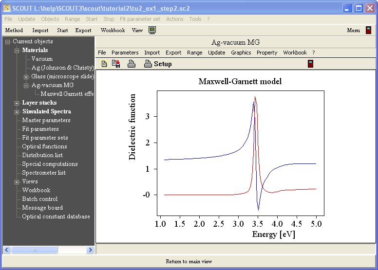
Note the sharp and strong resonance at 3.5 eV which is the frequency where the real part of the Ag dielectric function equals -2.

 

We are ready now to compute the first effective medium transmission spectrum. Drag the effective dielectric function 'Ag-vacuum composite' to the layer which contains still homogeneous silver and recompute the transmission spectrum:

The only parameters in the model that can be optimized are the film thickness and the volume fraction of the Maxwell Garnett model. Select both as fit parameters and use sliders to test the influence of each parameter on the transmision spectrum.

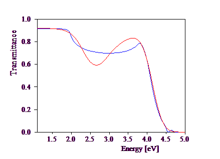
An automatic fit is quickly done and leads to the following 'agreement' of model and experiment:

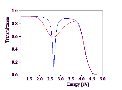
The thickness is 1.7 nm, the volume fraction 0.66 (which is too high for a reasonable application of the Maxwell Garnett formula). Looking at the spectra, it is obvious that the single resonance of the Maxwell Garnett model is too sharp.

As an exercise you can verify that also the other transmission spectra (2.std, 3.std, 4.std) cannot be fitted well using this simple effective medium theory.

The present configuration is stored as tu2_ex1_step2a.sc2 in the directory of this example.

 

Bruggeman formula

We can also try the probably most often applied effective medium model, the Bruggeman formula. Frequently this is called the Effective Medium Approxiamtion (EMA) as if it were the only one. This is very misleading. As you see in this tutorial, there are different effective medium concepts which differ in their spectral densities for a given volume fraction.

The spectral densities behind the Bruggeman formula are these:

 

 

At low volume fractions the spectral density is just a single peak which rapidly broadens with increasing volume fraction. The broadening is asymmetric. At f=1/3 the left side of the peak reaches n=0. For volume fractions above 1/3 there is a non-zero percolation strength (see the technical manual for an explanation of this term) contained in the Bruggeman formula:

 

 

The scenario of the spectral density development with increasing volume fraction is quite reasonable: Isolated particles get closer and closer as the density increases, and finally a connected network is built up. This qualitative behaviour makes the Bruggeman formula a good choice in many cases. However, there is no reason why a real system should exhibit an onset of a network at f=1/3 and why the percolation strength and the spectral density should follow the assumptions displayed above.

It is interesting to note that the original derivation did not assume a real geometric arrangement of the particles, but was based on some plausibility arguments. In particular, the percolation threshold at f=1/3 was not introduced on purpose. In fact, the Bruggeman construction leading to the formula (see the technical manual) did not consider percolation at all.

 

Let's now test the performance of the Bruggeman formula in the case of the silver layers on glass. Create an object of type 'Bruggeman model' in thematerial list and call it 'Ag-vacuum Bruggeman'. Set the parameters as you did in the case of the Maxwell Garnett formula, i.e. the volume fraction is 0.1, vacuum is the matrix material into which silver particles are embedded. With the main window's Range command you can set the spectral range for all objects that compute spectra, including the new Bruggeman effective dielectric function. This now looks like this:

 

 

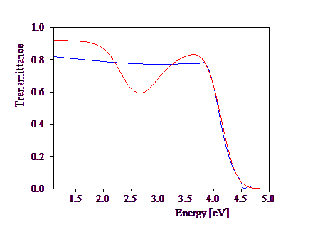
Compared to the Maxwell Garnett case much broader featues occur. This gives hope for a better agreement of measurement and model. To compute the 'Bruggeman transmission spectrum' the new Bruggeman object has to replace the former Maxwell Garnett entry in the layer stack. Recomputing the transmission spectrum you should find the following:

 

 

Adjusting the volume fraction and the film thickness as fit parameters the best result is

 

 

This could be considered a little better than the Maxwell Garnett solution but the agreement is far from being satisfying. The simulated absorption feature is now too broad.

After the optimization the volume fraction is 0.14 and a layer thickness of 20 nm is found. This configuration is stored as tu2_ex1_step2b.sc2.

 

Looyenga formula

Another simple effective medium concept with only the volume fraction as geometry parameter is the so-called Looyenga formula. This is interesting since it contains percolation for any volume fraction. The spectral density is this:

 

 

The percolation strength depends on the volume fraction as follows:

 

The required steps for testing this model should be familiar to you by now: Create the corresponding effective dielectric function object (type: Looyenga model) in the material list. Then open its 'parameter tree branch' and set the parameters appropriately. Set the spectral range and replace the Bruggeman entry in the layer list by the new Looyenga object. Then recalc and optimize the parameters.

Finally I got this:

 

 

You could have guessed the result already: The features of the spectral density are even broader than in the Bruggeman case and also the 'absorption feature' in the transmission spectrum is much too broad. Hence we have to conclude that this model is even worse than the previous ones. You can learn from this that you should not use a theory containing a silver network to describe an island film without connections between the silver particles.

This configuration is stored in tu2_ex1_step2c.sc2.

 

In the next step (applying a flexible model making explicitly use of the Bergman representation) we will achieve a much better agreement of model and measurement.