This very powerful action shows the influence of one of the model parameters on optical spectra. It works like this: In the main window of SCOUT, the command Actions|Parameter variation is executed. In a dialog you can pick one of the model parameters and set the range of the variation by specifying the minimun and the maximum value and the number of parameter values that you want to consider. For each particular value of the parameter range, SCOUT computes all spectra and stores them appropriately in worksheets in the workbook.

In most cases you want to inspect the results graphically. This can be done by copying the workbook data to the clipboard and from there to Excel or any other software of your choice, or you can do the visualization using the Collect object that is built in SCOUT.

Here is a step by step example. The goal is to investigate the dependence of a reflectance and an ellipsometry spectrum on a layer thickness. In order to concentrate on the demonstration of the parameter variation technique, a very simple example of a silicon oxide layer (layer type: thin film. This type of layer is automatically treated with coherent superposition of partial waves and the unit for the thickness is nm) on a silicon substrate (halfspace) is used. A reflectance spectrum (normal incidence of light) and ellipsometry data (70 degrees angle of incidence) are computed in the spectral range 400 ... 800 nm (100 spectral data points).

The individual steps are these:

Activate - in the main window of SCOUT - the command Actions|Parameter variation and observe that you enter this dialog:

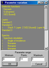
Select the layer thickness and a parameter range from 0 to 200 nm using 21 points (this means you will have 10 nm steps in the variation) according to the following settings:

If a parameter has a unit (like thicknesses) you have to specify the parameter range using exactly the same units. In the present example the unit of the layer thickness is nm.

After pressing OK SCOUT computes all the required spectra and automatically opens the workbook:

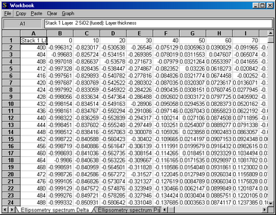
SCOUT has created a new worksheet for the reflectance data, and two new worksheets for the cos(delta) and tan(psi) values. Each worksheet has in its first row the name of the varied parameter and the parameter values. The first column downwards contains the spectral position (here the wavelength in nm). Below each parameter value there is a column with the corresponding spectrum.

Clicking in the gray field to the left of 'A' and above '1' selects the whole worksheet. The Copy command transfers the selected cells into the clipboard. From the clipboard you can get the data with Paste in Excel (or what ever program you prefer for data juggling).

If you like you can also generate 2D or 3D graphs with SCOUT which provides a built-in Collect object for doing this. The operation of this part of SCOUT is described in a separate section.

After you have done a parameter variation, you can apply the SCOUT command Actions|Repeat parameter variation to do it once more. SCOUT will empty all relevant worksheets and fill them with new data. You do not have to select the variation parameter and the range any more. This way to work is very useful in optimizing a model where you manually make frequent changes and you have to inspect the parameter variation after each modification of the model.