Navigation:  The optical model > Spectra > Reflectance, Transmittance, ATR > Introduction to spectrum simulations

Reflectance, transmittance, ATR and related spectra can be computed using objects of type 'R,T,ATR'. Opening these objects with a right mouse click in the treeview you get access to a window like this:

 

 

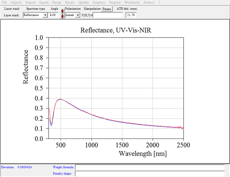
You have to set several items to uniquely define the spectrum to be simulated:

 

Layer stack

If you work with several layer stacks you have to assign the layer stack for this spectrum. Open the list of layer stacks with Objects|Layer stacks in the main window:

 

 

Start a drag&drop operation from the layer stack you want to use. Drop it onto the white field below the label 'Layer stack' in the spectrum window. Convince yourself that the right layer stack has been assigned after this action.

If you want to compute reflectance and transmittance spectra for laterally structured samples you can use spectra of type 'Layer mix' instead of the type 'R,T,ATR'.

 

Range

The Range command lets you define the spectral range of the simulated spectrum. As in previous SCOUT versions this range is not required to be the same as the one used for the dielectric function definitions.

 

Spectrum type

Here you can choose between different quantities that are computed. At present the following options are possible:

 

•Reflectance

•Transmittance

•ATR (attenuated total reflection)

•Absorbance ( = -log(transmittance) )

•Refl. absorbance ( = - log(reflectance) )

•1-R-T

 

Angle

This is the angle of incidence being zero at normal incidence of light and 90° at oblique incidence. As mentioned above the light is incident from the top halfspace of the layer stack.

You can also describe experiments where the illumination comes from the bottom of the the sample by setting the angle to a value between 90° and 180°. If you choose 172°, for example, the spectrometer beam comes from the sample's back with an angle of incidence of 180°-172°=8°.

 

Averaging over several angles of incidence

Sometimes it is important to average optical spectra for a distribution of angles of incidence. You can do this in SCOUT the following way. Open with Object|Angle of incidence distribution a list where you can define (by pushing the '+' button) as many angles of incidence as you like. Each angle gets a weight:

 

 

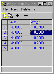
As soon as there is an entry in this list SCOUT ignores the angle setting in the spectrum window (see above) but computes for each angle in the list the spectrum. Each spectrum is multiplied by the weight of its angle of incidence. Then all spectra are added to the final spectrum which is displayed in the spectrum window. Note that the user, i.e. you, is responsible for the correct normalization of the weights (at least up to now). Of course, the sum of all the weight values should sum up to unity to represent a nice distribution function.

If you want to return to the normal setting of a single angle of incidence in the spectrum window you have to delete with the '-' button all entries in the list of angles of incdicence.

 

Polarization

For the polarization the following settings can be used:

 

•s-pol: S-polarization

•p-pol: P-polarization

•mixed: A user defined mixture of s- and p-polarization

 

Manipulation

After the computation of one of the spectrum types listed above you can apply a user-defined formula to finally modify the spectrum. By using a special keyword in the formula you can refer to the reference spectrum mentioned below. See the section on spectrum normalization for details.

 

Target spectrum

In addition to the simulated and the measured spectrum, you can display a target spectrum. This is useful if you use SCOUT for production control: In this case the target spectrum would represent the spectrum of the ideal spectrum, i.e. it represents what you wish to see for the production all the time. You can set the target spectrum in a separate object that you open with Objects|Target spectrum.

With File|Options|Target spectrum you can control how the target spectrum is displayed: Activate the checked menu item Show to show it, set the Pen to determine which pen is used to draw it, and select Line mode in order to set the line mode for drawing the spectrum.

 

ATR diel. const.

If you compute ATR spectra, the incident beam is incident from a material with an almost real refractive index which is higher than the  real part of the refractive index of the first material in the layer stack. You could replace the usual 'Vacuum' in the top halfspace of the layer stack definition by a suitable material and compute a regular reflectance spectrum. This is tedious and not very practical if you want to simultaneously analyze reflectance, transmittance and ATR spectra of one and the same sample. You would have to work with two different layer stacks in this case.

In order to avoid this complication, SCOUT lets you define the parameter ATR diel. const which is used only if you compute ATR spectra. In this case the top halfspace material assignment (usually Vacuum, as mentioned above) is ignored and a material with a constant and real dielectric function is used instead. The value of the constant real part of the dielectric function is given by the parameter ATR diel. const. The square root of this number is the refractive index of the ATR element.

Typical values are 11.7 for silicon and 16 for germanium in the infrared, or 2.25 for glass in the visible.

 

Import of experimental spectra

Experimental spectra can be imported using the Import command. After data import the experimental data are multiplied automatically by the spectrum defined in the Reference window.

 

Computing the deviation

The deviation of the simulated and measured spectrum is computed the following way: First for each data point of the simulated spectrum the value of the measured spectrum is computed by linear interpolation. The differences of the simulated and measured values are computed and stored in a data field which can be displayed together with the simulated and measured spectra. The display of the difference spectrum can be activated with the local file menu item File/Options/Difference/Show. The additional options Pen and Line mode regulate the style of the curve.

 

Without penalty shape function:

If no penalty shape function (see below) is defined, the difference value (simulated - measured) for each spectral point is squared. If a weight function (at the bottom of the window) is defined the value of the weight function at the spectral point is evaluated und used to multiply the squared difference. Finally the average of these numbers for all data points is computed. This is the deviation of this spectrum.

 

With penalty shape function:

In order to setup your own optimization strategies (especially for thin film design where you want to achieve certain spectral properties of a coating) you can define a so-called penalty shape function. This function is entered in a text field at the bottom of the spectrum window. In the user-defined formula you can use the symbol x to refer to the spectral position. The spectral unit is the same that is used for the computation of the spectrum, i.e. if you compute a wavelength spectrum in nm, x denotes the wavelength in nm. In addition, the symbol y represents the simulated spectral value, e.g. the computed reflectance or  transmittance value. Finally the symbol z refers to the difference of the simulated and measured value. You can use all the usual functions and expressions for penalty shape functions that are allowed for other user-defined functions as well.

The value of the penalty shape function is computed for each data point of the simulated spectrum and then multiplied with the weight function (if a weight function is defined). Finally the average value of the deviation for all spectral points is computed. This is the deviation of this spectrum.

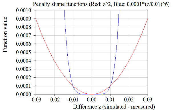
If the term z^2 is entered as penalty shape function, the computed deviation values are the averaged mean squared difference values that one would get without defining a penalty shape function (see above). The graph below gives a comparison of this "normal" choice (red curve) and a penalty shape function which tolerates differences below 0.01 but heavily punishes larger difference values:

 

 

 

Total deviation in the case of several spectra:

If the optical model contains several spectra the total deviation is obtained by adding up the deviation values of all spectra, multiplying each number with the weight that has been assigned to the corresponding spectrum in the list of spectra.

 

 

Special actions

Objects of type 'R,T,ATR' can perform some special actions which may be useful in some situations:

 

•Direct determination of layer thicknesses by the Fourier transform technique

•Data smoothing to reduce the noise in measured spectra