Navigation:  The optical model > Spectra > XRR

XRR objects are made to compute and fit X-ray reflectivity curves. XRR 'spectra' sometimes provide very useful thin film information, in addition to optical spectra. Analyzing interference patterns in the X-ray regime is simple and safe because the real part of the refractive index is almost identical to 1.

In order to combine optical analysis and XRR analysis in SCOUT or CODE you need to work with at least 2 layer stacks: one for XRR and a second one for the optical spectra. Layer thickness values must be synchronized using master parameters.

Defining optical constants for XRR computations means to set the real part of the complex refractive index to a value a little below 1, and the imaginary part to a very small positive value. The easiest way to do this is to use a susceptibility of type 'Formula for n and k' and fill in expressions like the ones shown below:

 

 

Since these 'optical constants' are used for a single energy only, it does not matter which spectral range you select for their computation.

 

The Range command of XRR objects lets you define the energy of the X-ray experiment in eV.

 

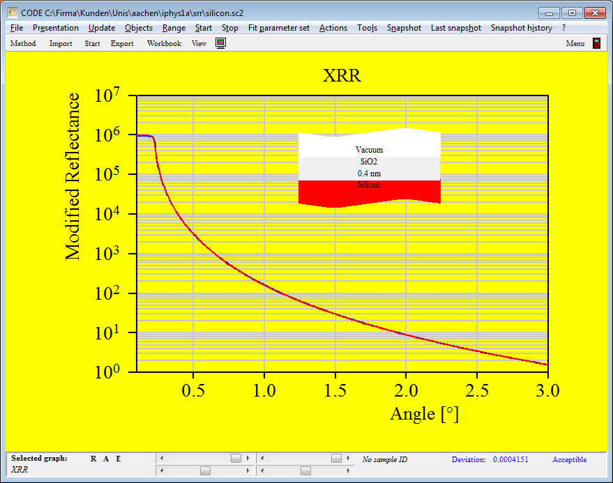
As a first simple XRR example the screenshot below shows XRR data of a SCOUT model for silicon (in blue) compared to measured data in red:

 

 

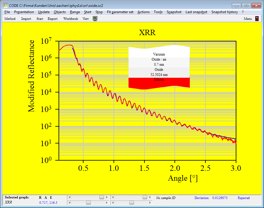
Here is a thickness fit of a SiO2 layer on silicon:

 

 

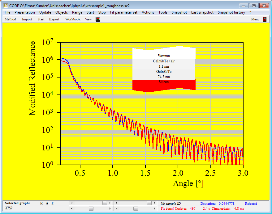
A thicker layer on silicon shows a typical problem at larger angles - the simulation is too high:

 

 

Introducing a slight surface roughness helps to improve the agreement of model and measurement: