Now we will add a cylinder to the scenery which is placed between the light source and the screen. The cylinder is going to represent an optical fiber used to guide light from one side to the other without reflection losses. This is achieved by making use of the total reflection of light that occurs if the angle of incidence is above the critical angle.

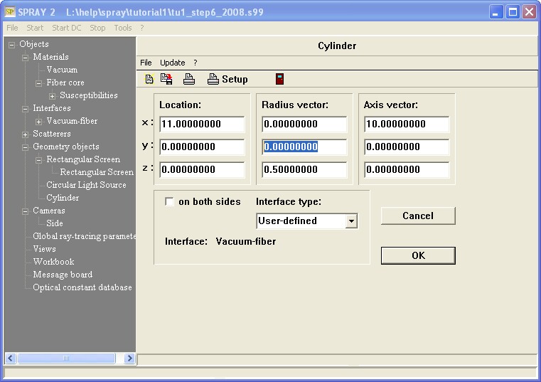
Open the list of geometric objects and create a new object of type 'Cylinder'. Name it 'Fiber'. To set its geometric parameters open it in the treeview:

The vector called 'Location' points to the center of the cylinder (drawn in blue in the sketch below). The 'Radius vector' (black vector) points from the center to the cylinder surface. It is perpendicular to the cylinder axis. The 'Axis vector' (displayed in red) is parallel to the cylinder axis and points from the cylinder's center to the center of one of the circular end areas:

The white area to the right of 'Interface' shows the name of the interface that is assigned to the cylinder. The default setting 'none' must be changed, of course. You do that by a drag&drop operation, dragging an interface from the treeview to the white area. The dialog above shows already all settings that are to be done in our case. Try to reproduce all values, in particular to drag the 'Vacuum-fiber' interface to the desired area. You have now defined a 20 cm long cylinder with 1 cm diameter, covered with an interface that represents the transition from vacuum to the fiber core material:

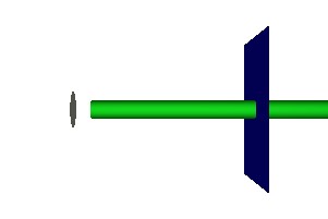
Looking at the rendered view called 'Side' we see the following situation:

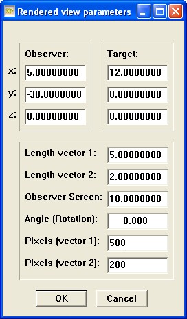
Move the screen to x = 25 cm and re-arrange the rendered view settings according to the following dialog:

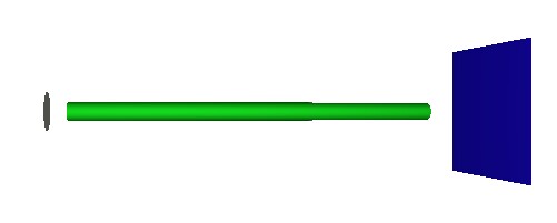
Now you can view the complete cylinder (after using the Draw command):

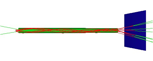
Try a few test rays and check (qualitatively) that the wave-guiding by total reflection works:

Now change the light source geometry: The location should be (0.5, 0, 0) (a little closer to the fiber head) and the radius is reduced to 0.2 cm. Now all emitted rays hit the fiber front end:

Go to the main window and press the 'Simulation' button to start a ray-tracing simulation. Look at the screen. It should have received roughly 92% of the radiation which is expected: The reflection losses entering the fiber are about 4%, and the same amount is lost at the other side.

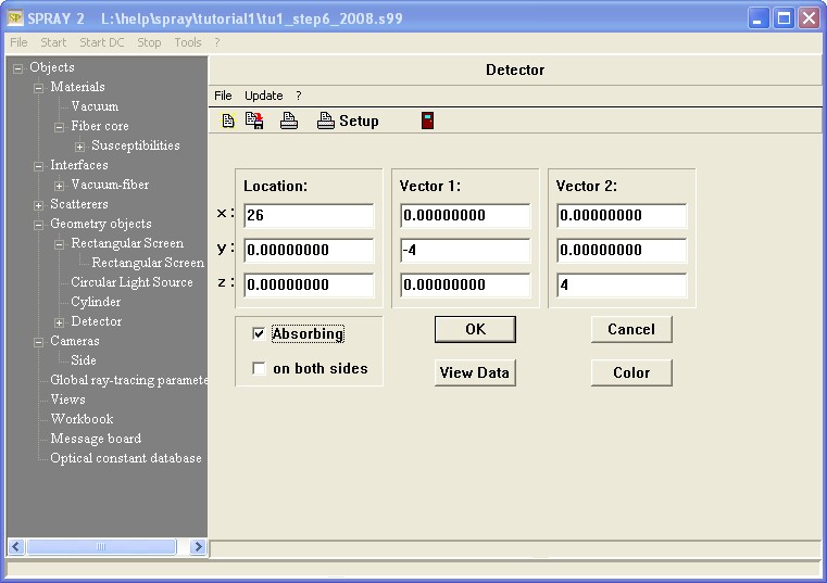
Since we want to be able to predict optical spectra we need to introduce a detector that records the amount of received rays for each spectral point. Open the geometric object list  and create an object of type 'Rectangular detector'. Name it simply 'Detector'. Like a screen, this is a rectangle counting how often it is hit by a ray. However, instead of saving the position of the hit point, it records spectral information. The fraction of received rays is recorded for each simulated spectral point. Place the rectangle a little behind the screen and give it the same size and orientation. Make sure that the surface normal points to the side of the fiber. The following dialog shows the appropriate settings:

Open the rendered view 'Side' and update the picture by the Draw command to inspect the setup:

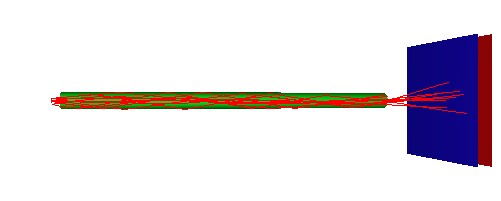
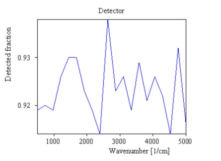
The detector is positioned to the right of the screen and will detect the rays passing the right end of the fiber and the screen. Now it is time to record the first SPRAY spectrum. In the main window, press the Simulation button. When the computation is finished, expand the 'Detector' treeview branch and right-click the subbranch 'Spectrum'. A new window opens displaying the recorded spectrum. Press the 'a' key on the keyboard to do an automatic scaling. The spectrum should be similar to this one:

Apply the command Graphics|Edit plot parameters and change in the following dialog the minimum and the maximum of the y-axis to 0.0 and 1.0, respectively. The parameter called 'Tick spacing' should be set to 0.2 . The graph changes to this:

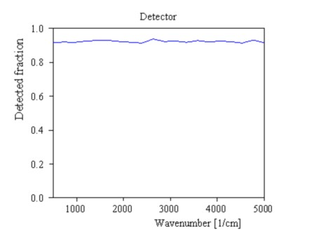
The spectrum does not show too much structure. In fact, it should be constant since no part of the present model contains any spectral variation. The variations in the spectrum are due to statistical noise. Remember, that we work with 1000 rays per spectral point. The expected noise has a level of about the square root of 1000 divided by 1000, which is - roughly - 3%. In the next step we will add an absorbing thin film to the model which will cause some more interesting features.

The configuration achieved up to now is saved as tu1_step7.s99.