First we will do some introductory exercises which do not require the definition of optical constants. The goal is to inspect the output of a point light source with a screen. This example is simple enough so that we can guess how the result should look like. If we trust the model we can extend and modify it. Finally we will be able to do advanced simulations which cannot be done easily otherwise.
Start SPRAY:

and press immediately F7 to enter the treeview level:

Right-click the branch called 'Geometric objects'. This command opens the object list in the right part of the main window. You can get general information on SPRAY lists in the technical notes section. The geometric object list is used to define the geometric objects in the setup. In between the '+' and the '-' button there is a dropdown list which is empty at the program start. Here you have to select the object type that you want to create. Select the entry 'Point Light Source'. Note that there is no object created yet. To do this you have to press the '+' button. A new object is created with a default name ('Point Light Source'). Click on the name and change it to a name of your choice, e.g. 'The lamp'. Press Enter, and the list now looks like this:

Note that the treeview branch 'Geometry objects' has a + sign to its left. You can expand this branch by a left mouse click on the +.
SPRAY setups have to have exactly one light source. The light source must be embedded in a certain material to have a well-defined starting environment for the rays. You have to set the light source material in a subwindow which also gives access to the geometric parameters of the object. You can open this subwindow by a right-click on the object's treeview branch:
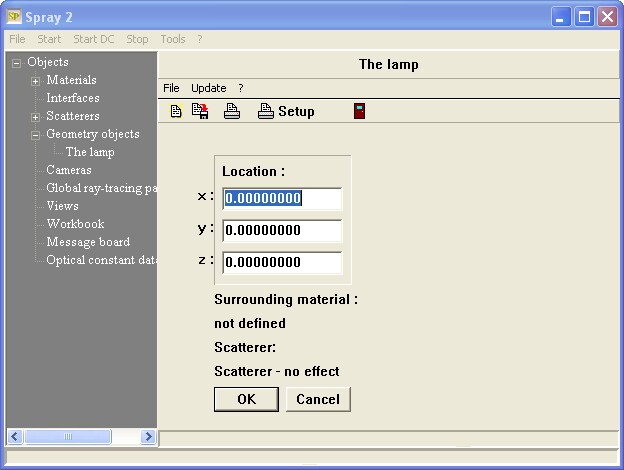
As you see there is not too much to do here. You can specify the x,y and z coordinates to define the position of the light source. We can leave the lamp at the origin for the moment, but we have to define a surrounding material. You have to do this by dragging a material from the list of dielectric functions (optical constants) to the text 'not defined'.
To get access to the list of materials right-click the Materials treebranch. The following list opens:

There is already the entry 'Vacuum' which we can use. To assign the material 'vacuum' to the point light source, proceed like this: Expand the treeview branch Materials so that the 'Vacuum' object appears in the treeview. Then right-click the treeview object 'The lamp'. Finally drag the 'Vacuum' object in the treeview to the text 'not defined' under 'Surrounding material'. Drop it there and verify the assignment:

Now we need an object to check if the light source works as expected. We will use a screen object to do this. Screens are very important to check a setup, so you should get used to apply screens right from the start. Go to the list of geometric objects (right-click the treeview item 'Geometric objects') and set the drop down list (Current entry is still 'Point Light Source') between the '+' and '-' buttons to 'Screen'. Then press the '+' button to create a new screen object. Open the new entry named 'Rectangular screen' by a right-click in the treeview:
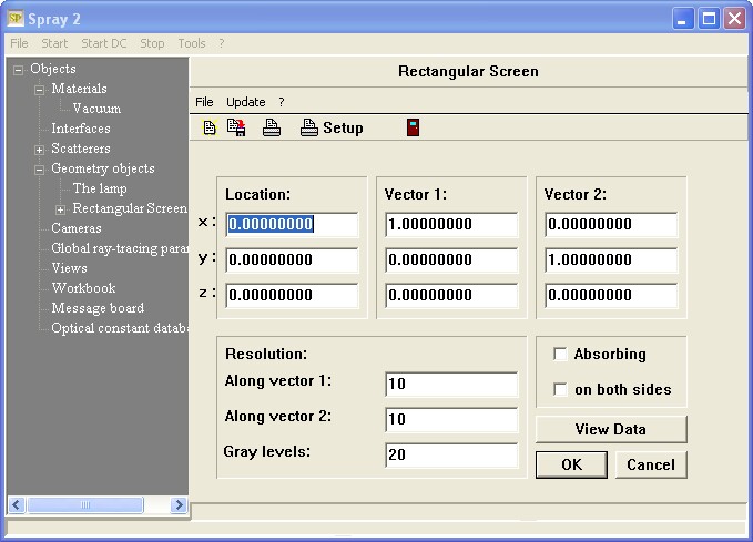
Compared to the point light source we have to set a lot more quantities to define the screen. The geometric position is defined by the center of the screen rectangle given by the x,y and z values of the 'Location' column (The blue vector in the picture below). The two other vectors (labeled 1st and 2nd) define the orientation and the size of the screen rectangle according to the following sketch:
The two vectors should be perpendicular to each other, their cross product defines the surface normal.
The parameters of the 'Resolution of Data' section define the number of pixels in the direction of the 1st vector (labeled as 'x') and 2nd vector ('y'), respectively. The 'Color' parameter determines the number of color levels for the graphical output. You will see immediately what this means.
During a simulation, screens count the number of rays that hit their individual pixels. The setting of the 'Absorbing' checkbox determines if the screen absorbs rays or not. If the screen is non-absorbing the rays are detected by the screen but continue their way as if the screen were not there. If 'on both sides' is checked the pixels count rays independent of their direction. Otherwise, only those rays that arrive from the surface normal side are detected.
To define a screen in the y-z-direction (dimensions: 8 cm by 8 cm) moved away from the origin by 10 cm in the x-direction you have to set Location to (10,0,0), 1st vector to (0,-4,0) and 2nd vector to (0,0,4). This way the surface normal points in the negative x-direction. Set the number of pixels in both directions of the screen to 50, the number of gray levels to 100:
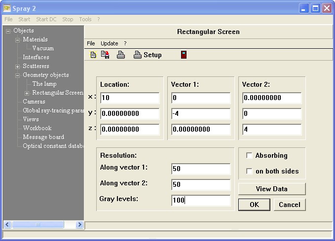
Press OK when you are ready with your settings.
Expand the object 'Rectangular screen' in the treeview and right-click its subobject (which is also called 'Rectangular screen'):
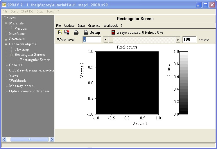
You see graphical representation of the screen. Since no simulation has been done yet, the screen is black up to now:
We are almost ready for our first simulation. However, before we start the computations right-click the treebranch 'Global ray-tracing parameters'. This opens a subwindow for setting some important quantities.
In the 'Spectral range' section you can set the spectral range for the ray tracing simulation. Specify the minimun, the maximum, the number of spectral points and the unit. For the latter you can choose between 1/cm (wavenumbers), nm (wavelength), eV (energy), micron (wavelength) and THz (frequency).
The 'Angle resolution' is important for interface objects. These compute (before the simulation is started) the angular dependence of the reflectance and transmittance using the specified number of points for the range 0 ... 180 degrees. Usually this does not take too long. Hence there is no reason to go to a low angle resolution unless you have a large number of interfaces in your model.
The 'Number of photons per spectral point' determines how many rays are processed for each spectral point. How many rays you need depends very strongly on the questions that you have to answer.
Finally you can set the 'Max. number of interactions' for each ray. After a ray has been emitted by the light source SPRAY counts how many interactions this ray has with the objects of the setup. If the specified maximum value of interactions is reached before the ray reaches infinity or is absorbed the tracing of this ray is stopped. This is to avoid situations where a ray is reflected back and forth forever between two ideal mirrors. Usually you do not have to change this value unless you study very special setups.
Set a spectral range of 500 ... 5000 1/cm (we will work in the infrared in the next steps) with 20 spectral points, 180 points angular resolution and 1000 photons per spectral point.
Before we start the simulation based on the present model you should save the complete SPRAY configuration with File|Save As in the main window. The present configuration can be found in the file tu1_step1.s99. If you have problems reproducing the next results please load this demo configuration and compare it to yours.
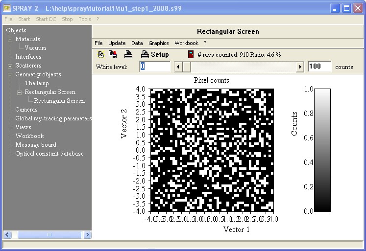
Now use the Start menu command to start the ray-tracing run. A progress bar tells you the present status of the computation. If it is finished you can look at the screen window to see how much radiation arrived. If this window is not on the screen any more you have to right-click it in the treeview:
If you like you can use the Graphics|Edit graphics parameters dialog to change the settings of the axis labels. Here is an example:
The graph now looks a little nicer:
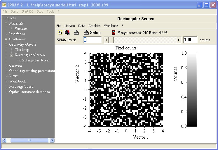
Screens are not wavenumber selective, they count every ray hit independent of the frequency. From the 20000 emitted rays 910 have reached the screen (4.6%). The distribution is quite uniform.
You can modify the scaling of the grayscale plot by moving the slider on top. The number to the left of 'counts' gives the number of photons per pixels which are plotted as 100% white.
Now we place the screen a little closer to the light source. The radiation distribution should be less uniform, with a higher concenctration in the center of the screen. More rays should hit the screen since it will cover a larger solid angle now.
Change the x-coordinate of the screen location from 10 cm to 1 cm (do not forget to press the OK button) and then press Start again. Now the screen looks like this (20 rays/pixel as 100% white level):

Note the larger fraction of rays reaching the screen (38.9%). This configuration was saved under the name tu1_step2.s99. If you cannot reproduce the above result, please load this configuration and compare it to yours.
Finally we can check if the screen gets 50% of the rays if it is placed very close to the light source. Since the light source emits isotropically half of the rays should hit the screen in this case. Set the x-coordinate of the screen's position to 0.001 cm and re-run the simulation. I found a value of 49.9% (tu1_step3.s99).