In many cases it is advantegeous to work with more or less collimated beams instead of point light sources. This is in particular important if you want to simulate only a part of a setup, e.g. a sample holder in a spectrometer. You could then start the simulation at an intermediate focus if you know the focus size and the beam divergence approximately.
In these cases you can use a light source of type Circular light source. Delete the point light source in the present configuration (by selecting its row in the object list and pressing the '-' button) and set the object type to 'Circular light source'. Create a new object of this type with the '+' button and open it (treeview right-click). Assign vacuum as surrounding material (see above how to do that by drag&drop) and set the radius to 1 cm. The dialog should now look like this:

This defines a disk with radius 1 cm at the origin, emitting rays in a cone of 20 degrees opening angle around the direction given by Surface normal (i.e. the positive x-axis).
Now move the screen to its original position at x = 10 cm and re-run the simulation. The screen looks like this now:

Almost all rays hit the screen now. This configuration can be found in the file tu1_step4.s99.
In addition to typing in geometry data to position your optical components in space you certainly would like to have a view on your setup. This can be done most conveniently using so-called camera views. These are 'snapshots' of your scenery which can be exported as bitmaps for documentation purposes. Here is a short introduction showing how to create and handle camera views.
Right-click the treeview branch Cameras. This list collects various views of your scenery. Select the type 'Rendered view' in the type selection dropdown list and create a new view object pressing the '+' button. Change the name of the new object to 'Side'. The camera list should now look like this:

Open the new object in the treeview:
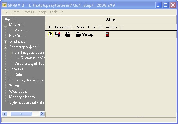
This window will show the view once it is computed. First we have to set a lot of parameters in the dialog that opens after the Parameters menu command:

The 'photograph' of the scenery is taken by an 'Observer' whose position is given by the vector called Observer. The observer looks towards a target point the coordinates of which are specified in the Target column.
Like in the following sketch there is a virtual pixel array between the observer and the scenery. The distance between the observeration point and the center of the screen is set by the 'Observer-Screen' parameter:

The horizontal extension of the screen is given by Length vector 1, the vertical one by Length vector 2. The screen is adjusted by 'gravity', i.e. the vector 1 direction is horizontal (perpendicular to the z-direction). However, if you like, you can rotate the screen by specifying an angle different from zero (parameter Angle).
Finally you have to set the resolution of the screen by specifying the number of pixels in the two screen directions. The more you take here, the more details you will see, but the longer you will have to wait for the computation of the picture.
If you set all parameters like in the dialog example given above you will see a side view of the scenery. After the Draw command the picture is computed and displayed in the rendered view window:
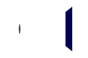
To the left you see the circular light source, to the right the screen.
In a rendered view, you can also have some action in the sense that you can emit some test rays from the light source and watch where they go. The '1' command sends 1 ray, the '5' command 5, and the '20' commmand sends 20, of course. You can execute any of these commands several times to accumulate as many rays as you like:
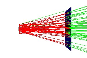
The rays that hit some of the objects are drawn in red, those that escape to infinity are drawn green.
If you want to clean a rendered view from the test rays you have to activate the Draw command ones more.
If you have specified more than one rendered view the test rays are drawn in all views simultaneously.
This configuration can be found in the file tu1_step5.s99.