Navigation:  User guide > Integral quantities in main window views

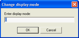
You can drag integral quantities like color coordinates from the list of integral quantities to a view list. If they carry a numerical value that value is displayed to the right of the name of the quantity. The format of the display is controlled by a mode parameter. If you select the view element and use the Edit command in the list of view elements, you are first asked to select the color for the text. Once the color dialog is closed, you are asked for the mode parameter in a dialog like this:

 

 

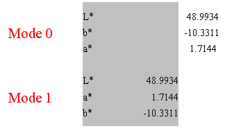
The name of the integral quantity (or the nickname, if you defined one) is shown, with left justification, inside the rectangle of the view element. If mode is set to 0, the numerical value is written to the right of the view object's rectangle, also left-justified. If mode equals 1, the numerical value is written right-justified with respect to the right side of the rectangle. Mode 1 is useful if you want to create tables of integral values in a view. The following example shows the difference between mode 0 and 1, with the gray rectangle indicating the width of the view objects' rectangles:

 

 

The following integral quantity objects are displayed in a special way when they are dragged into a view:

 

 

Color view

These objects are displayed in various ways, depending on your choice. You can display a colored rectangle, the color coordinates as text, a mixture of colored rectangle and coordinates as text, the color impression as text or the position of the color in x-y-plane.

The following graph gives an overview of the options on the right side:

 

 

The "color impression as text" mechanism uses the coordinates a* and b*. They are converted to a color name according to the following map:

 

 

 

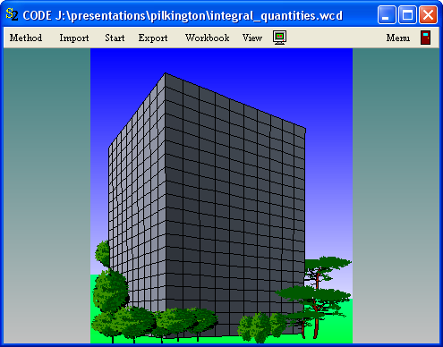
Virtual Office Tower

If you drag objects of type 'Virtual Office Tower' to a view be aware of the large computational work that has to be done to draw the image. The build-up of the view may take quite a long time on slow computers. Tower objects are drawn in views like this:

 

 

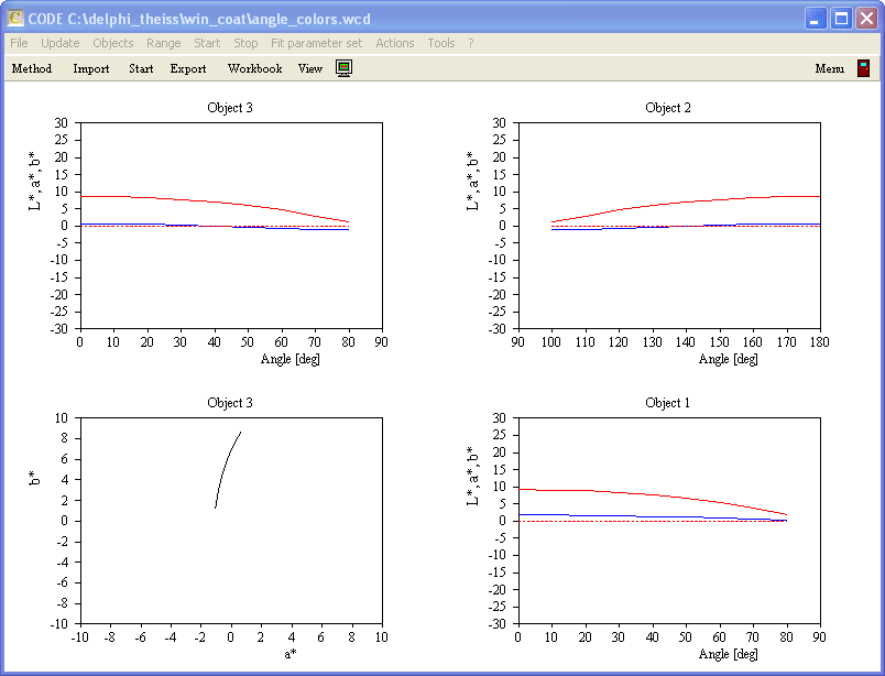
Color angle variation

Objects of this type are represented in views the same way as other integral quantities that produce a numerical value as output (see above, mode = 0 or mode = 1). If you set mode = 2 a graph is generated that fills the view element's rectangle:

 

 

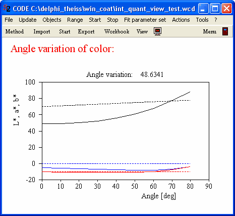
The graphics parameters used for the plot are set in the dialog that follows the objects Edit command (see above).

The solid lines in the graph represent the variation of L* (black), a* (blue) and b* (red) with angle of incidence. The dashed lines show the corresponding target values. If you choose to display the weight function (check the appropriate checkbox in the object's dialog) it is drawn green.

Setting mode = 3 generates a 'b* vs. a*' graph. The graphics parameters for this plot are also set in the Edit routine of the color angle variation object (see above).

 

You can generate several view objects that refer to the same color angle variation object like in the case below: The two graphs on the left show the same color angle variation object: