Color coordinates |
  
|
Color coordinates |
|
Color coordinates have several options which are set in the following dialog:

You access this dialog by selecting the color coordinate you want to change and activating the menu item Edit (or by clicking with the right mouse button on the color coordinate).
The following color coordinate types are implemented at present:
All are based on X,Y and Z which are computed using the selected illuminant and observation angle. As observation angle you can select either 2° or 10°. For these angles color matching functions are defined.
The illuminants called A, D65 and C are available for color computations. If you need more, you can import additional illuminants from an external file, including user-defined spectra. The file must be a text file with semicolon separated columns as it can be generated by Excel. An example of the import is given in the section Background/User-defined illuminants for color computation. The additional illuminants will show up in CODE color dialogs and can be selected in order to compute color coordinates. If you store a CODE configuration after you imported additional illuminants, the imported spectra will be stored as part of the configuration.
Color view
Color view objects can be used to roughly visualize the 'color' of a spectrum. With the Edit command in the list of integral quantities the following window opens:
The window shows (after selection of an illuminating spectrum) the computed color coordinates X,Y, and Z and converts these to L*, a*, b* and RGB coordinates (Red, Green, Blue). The latter are used to display the color in the upper right half of the window. Since the conversion from X,Y,Z to RGB values is not very accurate the color view should not taken too seriously. Most PC screens are not calibrated properly anyway. So take the color impression just as a rough indication of the real color.
For dark colors with low L* values the visualization is quite useless since the color appears to be black on PC screens. For such cases the bottom rectangle can be used to display a brighter version of the color: It shows a visualization of a color with the same a* and b* values, but a user-defined L* value. Use the slider position to vary L* from 0 to 100. Note, that you must use the Update command in the list of integral quantities or in the main window of CODE in order to re-compute the color coordinates after you have changed the slider.
You can leave the color view window open while you change the optical model, e.g. while changing film thicknesses with sliders: The visualization is updated whenever the model is re-computed.
Color view objects can be displayed in a view in CODE's main window (see below).
Color angle variation
This object can be used to inspect and optimize the variation of a coating's color with angle of incidence. For a user-defined angle range, you can set target values for L*, a* and b*. For each angle, the object will compute L*, a* and b* using the actual coating. The mean square deviation between actual and target values is computed as the final number. You can set 0 as target for this deviation, and let CODE optimize parameters like film thicknesses in order to minimize the deviation, i.e. to achieve the wanted angular color variation. Be aware that for large angles the polarization of the incoming beam is important - in most cases the choice of unpolarized radiation in the corresponding spectrum object is most useful.
A view object showing a color angle variation object can display the angular dependence of L*, a* and b*. This is described below.
The Edit action for objects of this type first opens dialogs for the nickname, unit, scaling factor and decimals. Then two dialogs for graphics parameters are shown. These parameters are used by view objects that display object of type 'Color angle variation' in the main view. The first dialog sets the parameters for displaying L*, a* and b* vs. angle of incidence (set mode=2 in the view object to show this graph):

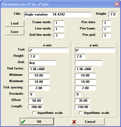
The second dialog sets parameters for a plot showing b* vs. a* (mode = 3 in the view object):
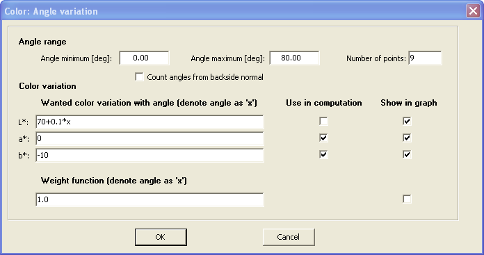
Then, in the final step, the following dialog lets you define the parameters of the computation:

In the top section the angular range is defined by setting the minimum and the maximum angle and the number of points used to scan the angle range. The example shown above means a scan of angles between 0° and 80° with a 10° resolution. If you check the option 'Count angles from backside normal' an angle of 0° means that the radiation is incident from the backside of the sample. In this case the scan from 0° to 80° covers incidence angles in the spectrum simulation object between 180° and 100°.
In the center section you can specify the wanted color variation with angle: For L*, a* and b* you have to enter an expression for the variation of the value with angle. The angle must be referred to as 'x'. The following example shows appropriate settings for a weak increase of L* with angle and constant a* and b* values:
You must enter a formula for the target values in each edit field before you close the dialog. Otherwise you will get a warning message.
The checkboxes labeled 'Use in computation' can be used to control if this quantity (L*, a* or b*) is taken into account for the computation of the deviation. In some cases it might be appropriate to leave L* out of consideration, and optimize only a* and b*.
If some angles are more important for the color appearance of a coating than others, you can express this using an angular dependent weight function. The squared deviation between actual and target values for each angle is multiplied with the weight function at this angle.
The settings of the checkboxes under 'Show in graph' determine wether this quantity is displayed in the view graph.
Color fluctuation
This quantity computes the variation of color in the case of fluctuating model parameters, such as thickness values. For each fluctuating quantity the color distance to the center color in L*a*b* space is computed for the upper and lower boundary of the fluctuation. The final value is the average color distance of all variations. This very simple computational scheme is used as a compromise between speed and accuracy.
In the case of large layer stacks with many fluctuating layer thickness values the use of color fluctuation objects may lead to quite large computational times. On the other hand, the design of 'stable' coating properties is quite easy with color fluctuation objects.
Dominant wavelength
The so-called dominant wavelength is computed by objects with the same name. Besides the computation of this quantity these objects also display the position of the color in the x-y-plane which is used to compute the dominant wavelength. With Edit or clicking the right mouse button a new window opens showing the following graph:

The blue line represents the position of pure spectral colors in the x-y-plane (380 to 700 nm wavelength). The black circle shows the position of 'white' whereas the blue circle shows the position of the current spectrum. If the model changes (e.g. by varying a layer thickness with a slider) the graphics is updated automatically: You can instantly see the blue circle moving through the x-y-plane. This is a very instructive tool for layer design.
Purity
This quantity closely related to the dominant wavelength is calculated by objects named 'Purity'. Purity objects feature the same graphics as dominant wavelength objects.