We are now ready to compute the reflectance spectrum of the model and compare it to measured data.

Open the list of spectra by right-clicking the treeview item 'Simulated spectra'. Rename the object 'Spectrum simulation' to 'Reflectance' by overwriting the entry in the name column.

The expand the list of spectra by a mouse click on the + to the left and open the 'Reflectance' object by a right-click. In the reflectance window, set the angle of incidence to 8°. Since the measurements have been done without polarizer you should set the polarization to mixed. In this case, s- and p-polarized spectra are computed and averaged with equal weight on both. Because there is no big difference between the s- and p-polarized cases at low angles of incidence you can just work with s-polarization for a little higher speed in the computation.

Set the Range to 200 ... 1100 nm using 100 data points and Recalc the spectrum. Modify the graphics parameters to achieve the following appearance:

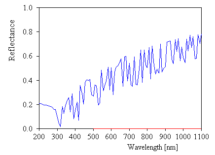
This spectrum looks a little strange, doesn't it? Something seems to be wrong. Import the experimental spectrum first.spc (SpectraCalc format) for comparison. Check carefully that the imported data have the range 200 ... 1100 nm. You should get

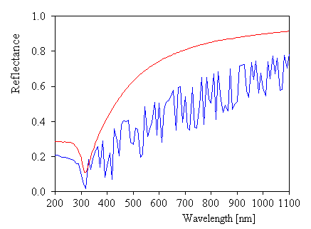
Note that the measured spectrum is smooth whereas the simulated one seems to be very noisy. Well, the reason for the 'noise' is the following: The simulated spectrum contains very narrow interference fringes due to partial waves reflected at the top and bottom interface of the glass plate. With only 100 data points between 200 and 1100 nm wavelength you cannot resolve the fringes. Hence you see 'random numbers'.

If you compute with high resolution you can clearly identify the fringes. Select a Range from 600 to 610 nm with 1000 data points, Recalc the spectrum and zoom in:

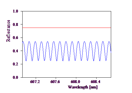
Nicely regular interference patterns show up.

Why don't we see such patterns in the measured data? There are several reasons for their absence. First, the resolution of the spectrometer may have been too low. In this case we have averaged over several interference fringes and get almost a straight line. In addition, the microscope slide has certainly a thickness variation over the investigated sample spot. This would also suppress interference fringes since you average over slightly different periodicities. The same effect would be caused by a beam divergence of the probing radiation.

To summarize: We have the strong wish to average over interference fringes in the simulation very much the same way the spectrometer does it in reality. It has been shown that there is a simple way to do it: Just switch in the layer stack from the 'coherent' to the 'incoherent' superposition of partial waves. Here is what you have to do. Open the layer stack window and click on the word 'coherent' in the glass layer:

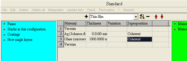
Press the F4 function key (or F5) on your keyboard. Note that the entry has switched to 'incoherent':

Close this window and go back to the reflectance spectrum. An Update shows that the noise is gone and we have hope to get something like the measured spectrum:

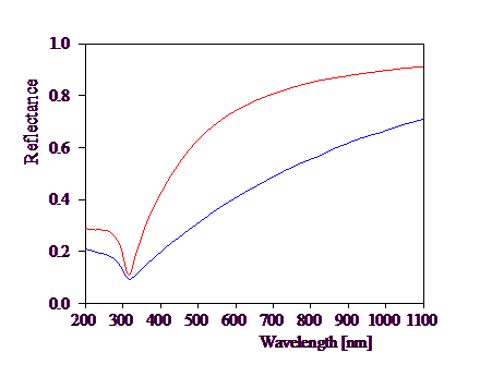
We are almost through: Select the silver layer thickness as the only fit parameter in the fit parameter list (you have learned in the previous examples how to do that) and Start immediately the automatic fit. Fitting the thickness in this case is so simple that the automatic fit works quite well:

Note the good agreement (except for a small remaining difference in the UV which is not important for the thickness results). The thickness that I found here is 20 nm.

As the final step you should use the main menu command Actions|Create view of spectra in order to show the reflectance spectrum in the main view.