Navigation:  Example 3: Photoluminescence spectra > Configuration of the PL object

Knowing the optical constants and the thickness of the porous silicon layer we can now try to compute a simulated PL spectrum. The corresponding PL spectrum objects are managed in the list of spectra, like reflectance, transmittance or ellipsometry spectra.

Start SCOUT and load the configuration tu2_ex3_step0.sc2 which holds the reflectance fit discussed above. Switch with F7 to the treeview level and open the list of spectra by a treeview right-click on Spectra. In the spectra list, create a new object of type 'PL spectrum': Set the dropdown box showing 'R,T,ATR' to 'PL spectrum' and press the '+' button to the left of the dropdown box. A new object is created and the list should look like this:

 

 

 

Right-click the PL-spectrum object in the treeview (expand the Spectra branch first):

 

 

Here we have to set a lot of parameters.

 

Excitation

In the 'Excitation' section the wavelength of the illuminating radiation and its angle of incidence and polarization must be specified. Take 457 nm, 0° and s-polarization.

 

Conversion

Here the properties of the PL layer are set. The layer stack is automatically set to the first layer stack in the list of layer stacks (which is the only one in most cases). Click on the small arrows to the right of the text 'Layer' to select the PL active layer in the layer stack. In the present case, there is only one layer possible which is the porous silicon layer, of course. The number of PL sources is set to 10 by default (see the SCOUT manual for an explanation of PL sources). Leave this number as it is for the moment.

The definition of the internal efficiency (see SCOUT helpfile for an explanation) is done in a separate window which opens with the button labeled 'Eff.'. It looks like this:

 

 

In this window, use the Range command to set a spectral range of 500 to 1000 nm with 200 points. The internal efficiency can be composed of several terms, e.g. several peaks, which are managed by a list called transitions. Open this list using the Transitions command. The list of transitions is almost identical to the list of susceptibilities which is used in dielectric function models. You can define several oscillators, for example, and their superposition determines the internal efficiency exactly like the imaginary part of the dielectric function. Create a Kim oscillator with parameters as shown in the following:

 

 

Up to now, all the oscillator parameters have to be specified in wavenumbers which is not convenient for PL spectra. This will be improved in the future. The value of 13500 1/cm for the resonance frequency of the Kim oscillator will roughly lead to a peak at 740 nm (where the maximum of the measured PL spectrum occurs).

Close the transitions list and compute the internal efficiency by the Recalc command. Press the key 'A' on your keyboard to autoscale the graphics. You should get this picture:

 

 

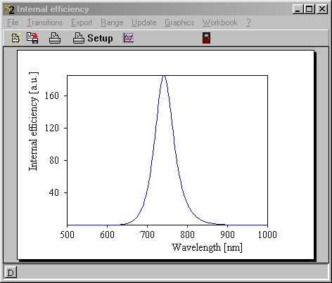
This will be our first approximation for the electronic transitions: one broad peak. You can now close the internal efficiency window.

 

Emission

Go back to the PL spectrum window and set the final quantities in the 'Emission' section: If you observe the PL radiation on the side from which the excitation is done set the  dropdown box below the text 'Emission' to 'Reflectance'. If you observe in transmission, choose 'Transmittance'. Select 'Reflectance' and specify 0° observation angle (the back-scattered radiation has been detected in this case) as well as s-polarization.

 

Finally, use the Range command to set a spectral range of 540 to 830 nm with 100 points. Now press 'A' to autoscale the graphics and see the following first simulated PL spectrum:

The model developed up to now is stored in the SCOUT configuration file tu2_ex3_step1.sc2.