Navigation:  Example 3: Photoluminescence spectra > Fitting PL spectra

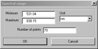
We can now try to fit the PL model to the measured spectrum. In the PL spectrum window, use the Import command to load the measured PL spectrum from the file tu2_ex3_pl.xy. Use the xy-format and make sure that the spectral unit of the imported data is nm as shown in the following screenshot:

 

 

Use the Graphics|Edit plot parameters command and set a range of 0 ... 6000 with steps of 1000 for the y-axis. Then press Update and see the following graph:

Obviously, the agreement of model and measurement is not satisfying yet. This will change soon.

 

In order to fit the PL spectrum only, go back to the main window of SCOUT and open the list of spectra with the menu command Objects|Spectra. In the spectra list, set the weight of the reflectance spectrum to 0 and keep the weight of the PL spectrum to be 1:

 

 

With this settings only the PL spectrum is used to fit parameters.

 

Again, go back to the main window of SCOUT and open with Objects|Fit parameters the list of fit parameters. Use the '- All' command to delete all fit parameters (which are left over from the reflectance spectrum fit). Then press '+' to select new fit parameters. In the list of possible fit parameters, go down to the spectra and select the first four parameters of the PL spectrum object (hold the Ctrl-key pressed down to select/de-select individual items in the list):

 

 

These are the parameters of the Kim oscillator that 'makes' the peak in the internal efficiency.

 

You are almost there. Go back to the main window and press the Start button to start the automatic fit. After a while the simulated PL spectrum approaches the measured one:

Note that the 'shoulder' around 620 nm is reproduced in the simulated spectrum - without adding an additional electronic transition. Open the internal efficiency window with the button labeled 'Eff.' and verify that it still contains a single broad peak:

 

The fit can be improved a little if the thickness of the porous silicon layer is fitted also. The PL spectrum has been recorded at a slightly different position as the reflectance spectrum. Hence the thickness in both cases may differ a little due to lateral sample inhomogeneities. Add the layer thickness to the fit parameters and press Start again to do the optimization of the model. The initial thickness of 1125 nm increases to 1128 nm which is a small difference only.

 

You can now do the following nice educational exercise: Open the PL spectrum and the internal efficiency window and arrange them on the screen such that both can be watched. Then create sliders (see the section about fit parameters in the SCOUT manual) for the layer thickness and the resonance frequency of the Kim oscillator, i.e. the spectral position of the internal efficiency peak. Move both sliders and investigate the influence of the peak.

The following graph (obtained with the 'parameter variation' feature of SCOUT) shows results for a thickness variation:

This once more stresses how important spectrum simulation can be for correct PL interpretation.

 

The final SCOUT configuration can be found in tu2_ex3_step2.sc2.