Spatial and time distributions, optical monitoring

Objects of type 'Electric field distribution' compute the spatial variation of the electric field amplitude in a layer stack. The main window of such an object looks like this:

el_field_1

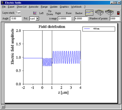
The graph means the following: The horizontal (x-) axis displays the position in the layer stack. The last interface to the bottom halfspace is at zero. Starting at zero and going to the right, you move through all layers until you reach the top halfspace. Each interface is indicated by a vertical black line. The light is incident from the top, i.e. the incoming wave approaches from the right with an amplitude of 1.

The example picture given above shows the situation for a 1 micron film (SiO2) and 400 nm wavelength: Above the layer (in the range 1 ... 4 microns) you see the superposition of the incoming and the reflected wave. In the layer (0 ... 1 micron) there is a superposition of all partial waves going from the right to the left with those moving from the left to the right. Below z = 0 there is only the transmitted radiation with a total amplitude that is constant in space.

________________________________________________

The following parameters determine the result of the electric field computation:

Layer stack:

The white text field to the right of the label 'Layer stack' shows the name of the layer stack for which the computation is done. You can change the selection of the layer stack by a drag&drop operation: Make sure the list of layer stacks and its subranches in the treeview are open. Open the electric field object with a right-mouse click (if it is not visible at the moment) and drag the wanted layer stack to the white text field where it is to be dropped.

Angle:

This is the angle of incidence of the incoming beam.

Pol.:

This is the polarization of the incident beam which can be s- or p-polarized.

z-range:

Here you specify the spatial range for the electric field computation by entering the minium and maximum z-values, and the number of points you want to use to sample the interval.

In the case of a 2D plot (like the one shown above) the z-range displayed may differ from the range in which values are computed. In all 3D plots the full computed range is shown always.

Range:

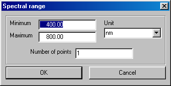
Using the menu command Range you can specify the spectral range for the computation. The usual dialog for spectral ranges is shown:

range_dialog

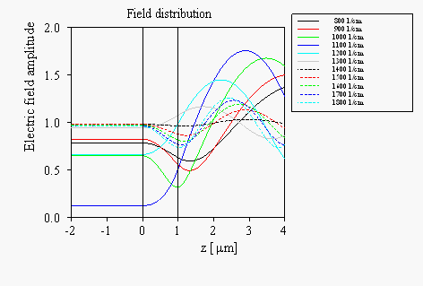
If the number of spectral points is set to 1 the electric field distribution is computed only for that spectral point. You can also use several spectral points to compute the field distribution for a whole sequence of spectral points.

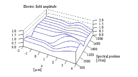
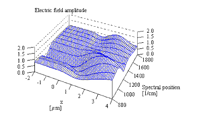
The following example shows the result for a 1 micron glass plate in the infrared (800 ... 1800 1/cm) using 11 spectral points:

clip0024

The individual lines are listed in a separate window which you can open using the Show list command:

spectra_list

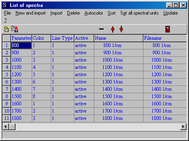
For each graph you can set the color and the line type that are used for the plot. You can type in new values or cycle through all values by right mouse clicks.

If the distribution is computed for several spectral points you can display the results also in 3D pressing the appropriate buttons. You can use a line plot with lines along the x-axis

clip0039

or a grid plot:

clip0040

Automatic re-computation

If the menu item File|Options|Automatic update is checked SCOUT re-computes the electric field distributions if the model is changed. This can be used to elegantly inspect the influence of a model parameter like a layer thickness or an optical constant parameter on the field distribution: Just move a fit parameter slider and instantly see what changes in the fields occur.

On the other hand, electric field computations and in particular 3D plots can consume quite a bit of time, and automatic re-computation should definitely be switched off during parameter fitting.

Export of numerical values

The computed distributions can be exported to convenient tables using the File|Report menu command. The numbers are written to the workbook which you can open by the command Workbook|Open workbook. You'll find the table in the worksheet called 'Last distribution'.

Important restrictions:

The present version of this object type requires that the transmission is slightly above zero. Otherwise you will get an error message and the computation is stopped. We are working on this problem.

Only coherent and isotropic layers are allowed at present.

No concentration gradient layers are allowed at present.