Fit parameters, sliders and 'fit on a grid' |
  
|
Fit parameters, sliders and 'fit on a grid' |
|
In the main window of SCOUT, switch with F7 to the treeview level and right-click the branch Fit parameters to open the list of fit parameters. At program start the list is empty. New parameters can be added using a dialog or by drag&drop from other lists of SCOUT.
Selecting fit parameters using the Fit parameter selection dialog
The New command (or the button labeled '+') of the fit parameter list opens a dialog with a list of all possible fit parameters from which you have to select. Dielectric function parameters (like resonance frequencies of oscillators or volume fractions of effective medium models), layer parameters such as thicknesses, fit parameters of the computed optical spectra (angle of incidence or constants that appear in modification formula) and master parameters are listed as follows:
As indicated, you can select many parameters simultaneously by pressing the Ctrl-key while clicking on the various lines. Clicking an already selected line 'unselects' it. Only those lines beginning with '>' represent fit parameters. The other lines contain guiding information only.
Selecting fit parameters by drag&drop
Instead of using the fit parameter selection dialog, you can also select fit parameters by drag and drop operations. You have the following possibilities:
•Drag a dielectric function from the dielectric function to the fit parameter list: All the parameters of the dielectric function are added as fit parameters.
•Drag from a susceptibility of a dielectric function model to the fit parameter list: All the susceptibility parameters are added as fit parameters. If you start the drag operation in a column that represents a value of a parameter (these columns are labeled as 'value') only that particular fit parameter is added.
•Drag a layer from the layer stack to the fit parameter list: All the parameters of that layer are added.
•Drag a spectrum from the spectrum list to the fit parameter list: All the parameters of that spectrum are added.
The fit parameter list
The chosen parameters are added at the end of the fit parameter list. This may look like this:
The name column gives the fit parameter's name. Since the names of fit parameters assigned automatically by SCOUT are sometimes quite lengthy you can overwrite the current name with your own. Just type in the new name. However, be sure to remember which parameter it really is. At present, there is no way to get back to the automaticly assigned name. In case you forgot what the parameter means, you have to delete it and create it new.
The Value column displays the current value of the parameter. If you would like to set bounds for the fit parameter value you can set an interval of allowed values using the Low limit and High limit values. The default values for Low limit and High limit are both zero, i.e. there is no variation at all. You have to set reasonable values manually with one exception: Starting with object generation 4.77 you can set Low limit and High limit automatically for thickness values when you create new fit parameters. Use the menu command File/Options/Fit to open this dialog which lets you set various parameters that control parameter fits:
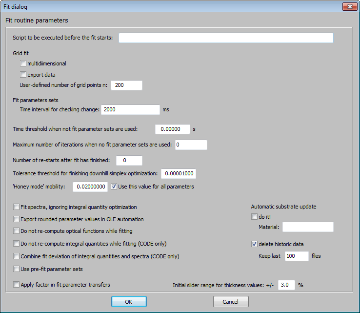
In the lower right corner you can set automatic limits for new thickness fit parameters. The value of the slider range is saved as a global default values in the default_values.ini file. It is not part of a specific configuration file but valid globally for all your work. The values is loaded when you start SCOUT, and saved when you shut down the program.
As Factor you can enter a number which is used to multiply the original value of the parameter: You can use this factor to scale up or down a parameter. If, for example, a thickness is given in micrometer you can multiply it by 1000 in order to see the value of the thickness in nm. If you change the factor, the current values of Low limit and High limit are multiplied by the factor as well.
Finally Digits specifies the number decimals used to display the current value of the parameter.
The Variation column allows to switch between different optimization options. In order to change the current option place the cursor on the cell and press the F5 key on your keyboard several times. By this action, you cycle through the available options. Stop where you want to stop. Pressing F4 you cycle backwards. At present, the following options are implemented in SCOUT:
Downhill simplex |
The parameter is optimized in the automatic fit according to the downhill simplexscheme which is used at present as optimization technique in SCOUT.
|
Frozen |
The parameter is not varied at all. This can be used, if you want to keep the parameter's value fixed for the moment but you may need it soon again. In this case, you don't delete the parameter but set is variation option to 'Frozen'.
|
Grid (100 points) |
If the variation option of a parameter is set to 'Grid (x points)' SCOUT will try x values of the parameter equally distributed in the range between Low limit and High limit before the automatic fit applying the downhill method is performed. For each value the model is re-computed, and the parameter value with the lowest deviation (i.e. difference between model and measurement) is taken as starting value for the automatic fit. If several fit parameters are to be varied on a grid of test values, the option 'Multidimensional grid fit' (please check or un-check this option using the menu command 'File|Options|Fit|Multidimensional grid fit' in the main window) determines how the computations are performed.
Multidimensional grid fit switched off: SCOUT will do one-dimensional grid variations in the sequence given by the fit parameter list, starting at the top. Note, that the result for the parameters' starting values will depend on the sequence. Hence, the choice of the grid variation must be done carefully.
Multidimensional grid fit switched on: SCOUT will collect all fit parameters for which a grid variation is set in the variation column, and do a multidimensional grid fit taking into account all possible combinations of parameter values. Note that the amount of computational work can be huge: If you select 4 parameters with 100 grid values for each of them, there are 100000000 re-computations of the optical model to be done. With multidimensional grid fit switched on, you can systematically scan a parameter space in several dimensions and hope to find the absolute minimum of the fit deviation. Setting the option 'File|Options|Fit|Export multidimensional grid fit data' you can log the fit deviation. For each point which is tried in the grid fit procedure the parameter values and the corresponding fit deviation is written to a text file. The filename is specified when you start the fit. The content of the text file can later be used to visualize the 'parameter landscape' which might be helpful in finding promising parameter values.
|
Grid (50 points) |
see above
|
Grid (20 points) |
see above
|
Grid (10 points) |
see above
|
Grid (n points) |
This grid fit uses a number of grid points that can be set by the user. You can define the number executing the menu item File/Options/Fit. The dialog that appears lets you enter a value for n in the section 'Grid fit'. There is a single number only - you cannot define different values for different fit parameters. |
Start at low limit |
Takes the lower limit of the parameter interval as start value for this parameter. Then continues like 'Downhill simplex' as explained above. |
Start at interval center |
Takes the center value of the parameter interval as start value for this parameter. Then continues like 'Downhill simplex' as explained above. |
Start at high limit |
Takes the upper limit of the parameter interval as start value for this parameter. Then continues like 'Downhill simplex' as explained above. |
Empty cell |
Here you can enter a formula to compute the value of the fit parameter. In the formula, you can refer to the values of the master parameters (see below). This way you can introduce relations between parameters, or control several parameters of the model by one master parameter. If you know, for example, how the parameters of your optical constant models depend on temperature, you could introduce the temperature as master parameter and update the optical constants while the temperature is fitted. |
Honey mode |
The purpose of this variation mode is to enable fitting with small variations around the current parameter values. It works like the downhill simplex mode with automatic limitation of the parameter range. When the fit is started the parameter automatically gets a low and high limit, based on the actual value p0 of the parameter. The range is controlled by a value called 'Honey mode mobility' - a value of 0.02 means that the high limit is 1.02*p0 and the low limit is 0.98*p0. These limits are active as long as the fit runs. If you press 'Stop' and then 'Start' again, then new limits are computed. You can set values for 'Honey mode mobility' for each fit parameter individually (use the local menu command "Honey mode mobility" of the fit parameter list). Alternatively, you can also set a global value for all parameters in the main menu with "File/Options/Fit": Set the value and activate the checkbox for global use of this parameter. |
The following example shows a frozen fit parameter and a factor different from 1.0:
Set fit parameters manually
You can do a 'manual fit' by typing new values for the fit parameters and selecting Update in the menu. This activates a new computation of the dielectric functions and all computed spectra as well as an update of all windows. This way you can immediately inspect how your changes influence the results.
Visual parameter variation: Sliders
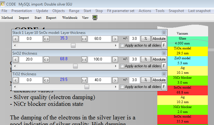
A much more elegant way to visualize the parameter influence on the spectra is the use of sliders. Select a fit parameter in the list and click on the Slider menu item. This way a new window is created and displayed on the screen that allows you to 'move' a parameter value with the mouse and see instant updates of the model spectra:

In the top of the window there are three values: The left and the right define the interval of the slider, the center one (in blue) is the actual value of the fit parameter. When the slider window is created the first time the slider range is the fit parameter interval Low limit ... High limit if you defined one. If you did not set a fixed interval for a fit parameter the initial range of the slider is 80 ... 120% of the current parameter value.
At any time you can overwrite the slider range by typing in new values for the left and right limit. If the slider position reaches the left limit, for example, you can also press the arrow labeled '<' to the left. This centers the limits around the actual parameter value. This operation can be used to work in a large parameter space without switching between mouse and keyboard. It works in the analogous way on the right side of the parameter range.
Pressing the button labeled '<>' expands the current parameter range by a factor of 2 and centers around the current value. The '><' button reduces the range to 50% and centers around the current parameter value.
In the upper right corner you can set slider limits in other ways: Clicking the % button sets the left limit to 97% and the right value to 103% of the current value. A click on the Absolute button set the limits to (current value - 3) and (current value + 3) (nm in this case). If you activate the checkbox Apply action to all sliders and click the % or Absolute buttons then all sliders get the corresponding limits.
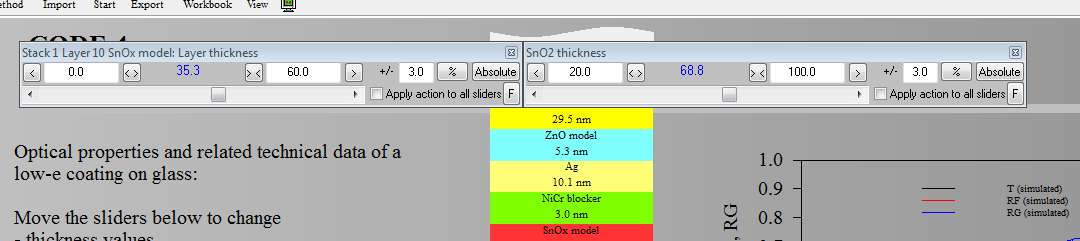
In addition to the Slider menu command you can also click on the fit parameter with the right mouse button to create the corresponding slider. You can open as many slider windows as you like if you want to investigate many parameters at a time. You can create regular blocks of slider windows by Drag&Drop: Create the first slider the regular way (as described above). To place a second slider window below the first one, 'drag' a fit parameter from the fit parameter list to the already existing slider and release the mouse cursor in the left half of the slider window. A new slider is created and placed directly below the first one:
If you release the mouse button in the right half of an existing slider the new slider window is created to the right of the existing one:
If you have several sliders scattered around on your desktop you can select one which should be the top slider of a new block and then click the F button: The other sliders will be positioned underneath the first 'master' slider.
Special slider features:
•You can create a slider by dragging a fit parameter from the fit parameter list to a spectrum simulation window. In this case the upper left corner of the new slider window is at the mouse cursor position.
•You can drag any susceptibility parameter that appears in a susceptibility list of a dielectric function window to a spectrum simulation window. The parameter is added as fit parameter to the fit parameter list and a new slider is created at the cursor position.
•You can transfer the fit parameter ranges that you specified in the sliders to the fit parameter list by the menu command 'Limits from sliders'.
Fit one parameter on a grid
The command Fit on grid can be used to optimize one of the fit parameters on a grid of test values. To do so, select the fit parameter that you want to optimize in the list. Specify a parameter range by setting the low limit and the high limit for this fit parameter appropriately. Then apply one of the commands Fit on grid|with 10 points, Fit on grid|with 20 points, Fit on grid|with 50 points or Fit on grid|with 100 points. Now SCOUT scans the parameter range using the given number of points and returns the best value of the fit parameter on that grid.
The command Fit on grid|Do all grid fits will start the grid optimization taking into account all fit parameters for which a grid fit has been selected in the variation column.
This 'fit on a grid' is good for a rough parameter pre-selection, for example for finding film thicknesses in the case of interference patterns. Afterwards you should use the automatic fit for further optimization of the model.
The submenu "Actions"
This selection of commands offers some shortcuts that turned out to be practical:
•Set all to 'Frozen': Sets all fit parameters to the state 'frozen'
•Set all to 'Downhill simplex': Sets all fit parameters to the state 'Downhill simplex'
•Set all to 'Honey mode': Sets all fit parameters to the state 'Honey mode'
•Set active material: Here the user can enter the name of a material which is then marked as 'active material' for the actions below
•Select all parameters: Take all possible fit parameters of the active material and select them as fit parameters
•Select oscillators: Selects all oscillator parameters of the active material as fit parameters. This is useful while adjusting models for organic materials in the infrared which may may have many oscillators. Manual parameter selection is tedious in such a case. Please note that for Kim oscillators (which are very much recommended) the parameter 'Gauss-Lorentz switch' is not selected since we found that in almost all cases absorption bands have a Gaussian line shape which is the default setting of Kim oscillators.
•Select oscillator strengths: Selects all oscillator strengths of the active material as fit parameters