To adjust the model to fit experimental data you could change the values of the model parameters in those lists where you defined them. It is more convenient, however, to collect these parameters in one single list which is called the list of fit parameters. Open this list by a right-click on the treeview branchFit parameters. The following (empty) list shows up:

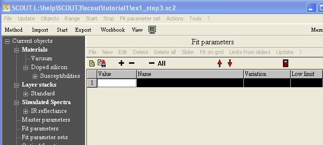
Pressing the + button or using the menu command New of the list (i.e. in the local menu underneath the Fit parameters title) you get a dialog box listing all possible fit parameters. First the list displays all dielectric function parameters, followed by the layer parameters. Finally the parameters of the computed spectra and the so-called master parameters are given:

Press the Ctrl-key down and click on those parameters that you want to adjust. In our example, select the plasma frequency and the damping constant of the Drude susceptibility that was named 'Carriers':

Leave the dialog pressing Ok and see that the chosen parameters are now in the list of fit parameters:

Manual fitting

First you can try some values for the parameters by typing in new numbers in the 'Value' column and active the Update menu command. SCOUT recomputes all windows that may have changed and you can inspect the new model, e.g. by looking at the reflectance spectrum. Try 3000 1/cm for the plasma frequency. The new spectrum (visible by a right-click of the IR reflectance treeview item) is this:

With a value of 5000 1/cm for the plasma frequency you get this:

Keeping the 5000 1/cm for the plasma frequency and increasing the damping constant to 500 1/cm the model spectrum is already quite close to the measured data:

Visual fitting

There is a much more elegant way to adjust parameters, namely by using sliders. Select the plasma frequency in the fit parameter list and create a slider with the Slider command or clicking on the parameter with the right mouse button. A new small window pops up:

With the mouse you can drag the plasma frequency between the limits given in the upper left and right corners. The present value of the fit parameter is given by the center value. While you move the slider all windows which need an update are instantly following the new values (if your PC is fast enough).

You should create two sliders for the plasma frequency and the damping constant, place them beside or below each other on the screen and play for a while with different combinations of the parameters - this way you get a good insight into the influence of each parameter on the spectrum. In our case it would be very instructive, for example, to have the two sliders, the dielectric function of doped silicon and the reflectance spectrum all together on the screen.

Automatic fit

After you have found a reasonable agreement of model and measurement in the manual or visual way you can try a completely automatic fit. In a simple case like the present one the optimization routine used by SCOUT should have no problem to achieve the best fit solution in a very short time. Just activate the Start command in the main window of SCOUT to start the automatic parameters adjustment.

Starting with values of 5000 and 500 1/cm for the plasma frequency and the damping constant, respectively, it should be no problem to reach the following agreement in a very short  time:

If you like to pass the results to other programs, you can generate a table in the SCOUT workbook. Right-click the treeview branch Fit parameters and use the local menu command File|Report. The data are written to a workbook sheet and the workbook is opened:

In the workbook you can select the cells that you want to transfer and use the Copy menu command (note that the Windows command Ctrl-C may not work here).

From these numbers you can compute (following the expressions given above) the desired quantities characterizing the semiconductor's charge carriers.

If you want to continue with the next example you should save the SCOUT configuration that you have obtained up to now. We will need it later.