Now you have to tell SCOUT which spectra you want to simulate and compare to measured ones.

Open the treeview branch Simulated spectra by a right mouse click:

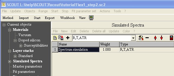
There is a pre-defined spectrum called 'Spectrum simulation' which is of type 'R,T,ATR'. As long as you just need to compute one spectrum you can use this pre-defined one. If you need more you have to create more.

In this example we are just going to compute one reflectance spectrum in the infrared. Select the name cell which says 'Spectrum simulation' at the moment and change its name to 'IR Reflectance'. Then click the + to the left of the treeview item Simulated spectra to open the corresponding subbranch. In this subbranch, right-click the branch named IR reflectance:

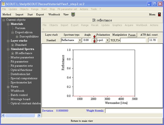
Here you can set the details of the spectrum that is to be computed. Leave the spectrum type 'Reflectance' unchanged, but set the angle (of incidence) to 30 degrees. All other settings can be used as they are except the spectral range. With the Range command you get the same dialog for specifying a spectral range for an object as we have used already in the definition of the dielectric function. Set the range to 100 ... 3000 1/cm with 100 data points. This range must not be the same as that used for the dielectric function, but it is reasonable to work with the same range in this case. After leaving the range dialog the spectrum is automatically computed. Whenever you change a parameter and you want a recomputation of the spectrum you can use the Recalc command.

Use the menu command Graphics|Edit plot parameters and set the graphics parameters as shown below (see the 'Graphics course' in the SCOUT documentation for a description of graphics parameters):

The spectrum should now look like the following:

Now, since the simulated spectrum is available, it is time to load the experimental data. With this tutorial a measured spectrum is distributed that we can use to practise. The filename is tu1_ex1_exp_data.spc and it is located in the subdirectory 'SCOUT tutorial 1'. After activating the menu command Import|from file of the reflectance spectrum object you have to select the SpectraCalc file type since the data are stored using this file format:

After this dialog the datafile is opened and some information about the found data is given in this dialog:

Do not change anything here except the unit if it is not correct. The units of the measured data and that of the simulation must agree (1/cm in this case).

After successful import the measured data are displayed in red together with the simulated spectrum in blue:

For the computation of the deviation between simulation and measurement it is important that for each simulated spectral point there are measured data (which may be obtained by interpolation, however). Hence you have to change the range of the computation, for example to the new range 600 ... 5000 1/cm. Instead of setting a new range  for the reflectance spectrum and also for the optical constant model individually you can due that in one step, globally in the main menu on top of the SCOUT window. There you find also a Range command which shows in a dialog the range of the first spectrum in the spectrum list. You can set the new range here and after you leave the dialog all spectra and all dielectric function models are re-computed using the new range. Set a new global range from 600 to 5000 1/cm with 100 points:

In addition, use the Graphics|Edit plot parameters command of the IR reflectance object to increase the range of the x-axis like the following:

Obviously, the agreement between model and measurement is poor and we have to change the model to improve it. We will do that now in the next step.

It would be nice to see the spectrum object in the main view which is displayed when you load a SCOUT method. Please read the 'Quick start ...' section of the SCOUT technical manual for a short introduction into view setups (or read the section about views for all details). In this first tutorial it is sufficient to see the spectrum object in the main view. You can achieve this by simply activating the main menu command Actions|Create view of spectra. Press F7 to switch from the treeview level to the main view level and convince yourself that the main view now looks like this:

Press F7 again to go back to the treeview level for the next step.