Multiple spectra view |
  
|
Multiple spectra view |
|
In configurations like this
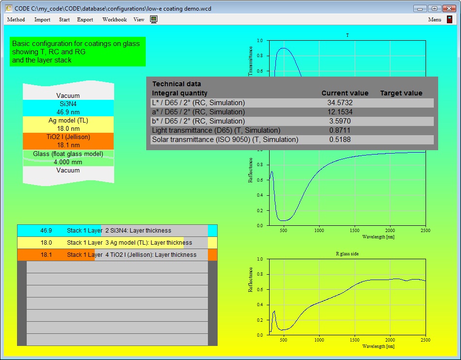
you might want to save some space. You can do so by using a view object of type 'Multiple spectra view' which displays many spectra in one graph.
You can display 2 sorts of data: Dynamic (i.e. eventually changing) spectra of the current optical model (all spectra in the list of spectra, but also optical constants of materials in the list of materials) and static spectra imported from data files.
Multiple spectra view objects show all spectra in a single graph. The settings are defined in a window like the following:
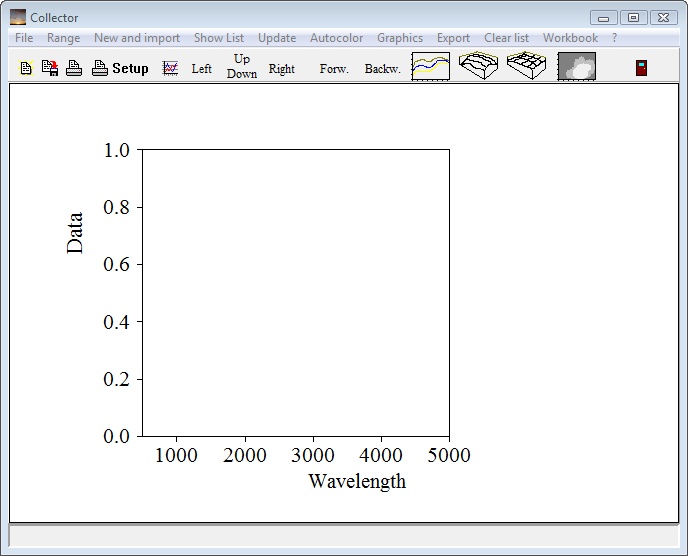
Using the Range command you define the spectral range of the displayed data. If the source data (see below) are defined in a different range (even with a different spectral unit) the data required for the display are generated by interpolation. Once the data are computed they are displayed using the current graphics settings (defined in the Graphics submenu). The graphics settings including the axis definitions can be done independently from the spectral range used to compute the data.
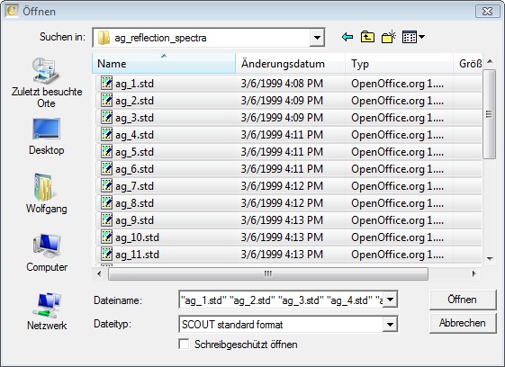
Importing external spectra
External spectra can be imported using the command 'New and import'. You can select multiple files to be imported. If you do so, it is recommended to click the last spectrum first in the file dialog and then move to the first spectrum, clicking it with the Shift key hold down. This way the order of the files is preserved which may be important for the following actions:
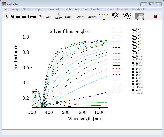
After data import and defining appropriate graphics settings the graph may look like this:
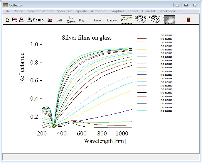
Since all spectra have the same label, we have to do some more work. Click on Show list to open the internal list of spectra of the object:
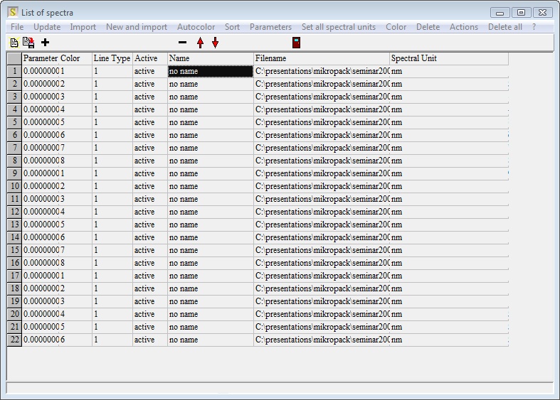
As a first action we can use the command Actions/Set filenames as spectrum names. This way the 'no name' labels are replaced by the filenames. Clicking on Autocolor (which assigns colors and line types automatically) and File/Options/Use control characters when drawing text (this option regulates the use of the underscore character) one gets the following graph:
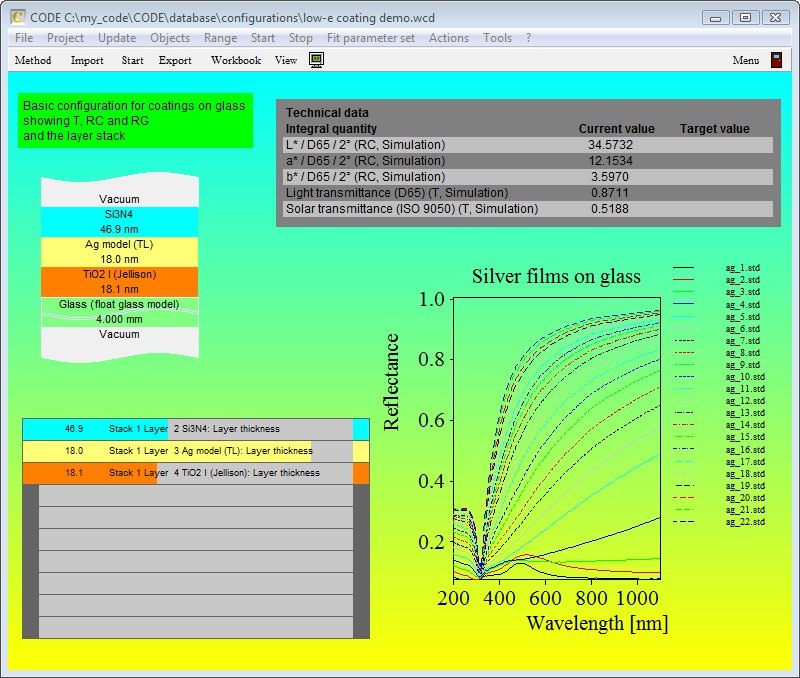
In the main view this would look like this:
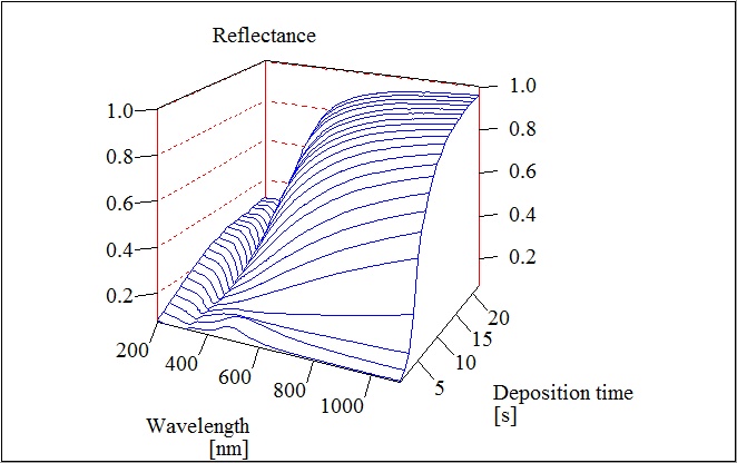
As you may have seen there are also symbols indicating that you can generate 3D graphs. In order to do so, the position of the spectra on the so-called parameter axis must be defined by a number called 'parameter'. This can be a temperature, a partial pressure of a reactive gas or, as in this case, the deposition time. Open the internal list of spectra to type in the parameter values in the first column. You can save a lot of typing work, if the spectra are already ordered in the list. Then apply the command Parameters/Set to 0, 1, 2, 3, ... or Parameters/Set to 1, 2, 3, ... to set parameter values automatically for the whole list. You can modify existing parameters using the commands Parameters/Multiply by constant factor and Parameters/Add offset. If, after your manipulations, the parameters are not ordered any more you have to apply the command Sort. Then you are ready to click on one of the 3D graph symbols to get a display like this:
of a false color plot like this:

False color plot use a color gradient starting with the color of the grid pen (yellow in this example) and ending with the color of the data pen (blue).
Displaying dynamic model spectra
Besides showing data from external data files, multiple spectra view objects can also display spectra that change as part of the optical model. In order to display the data of an existing material or spectrum object you have to specify the name of the object in the name column. In addition you have to indicate the wanted spectrum.
Available spectra for reflectance and transmittance objects are
o(simulated): refers to the simulated spectrum
o(measured): refers to the measured data
o(target): stands for the target spectrum
o(reference): for the reference spectrum
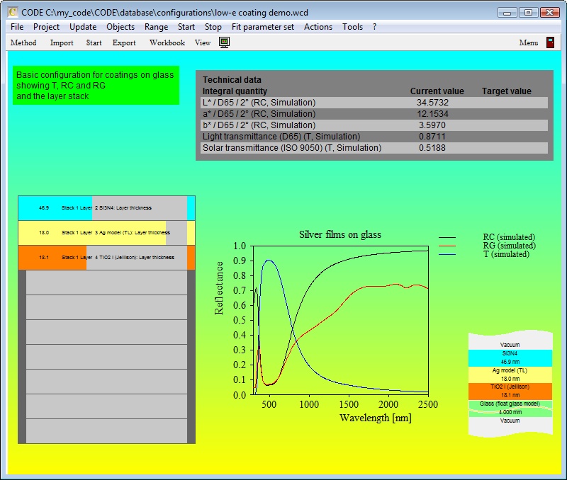
Valid names are then RC (simulated) or T (measured) if objects in the list of spectra named 'RC' and 'T' exist. Here is an example
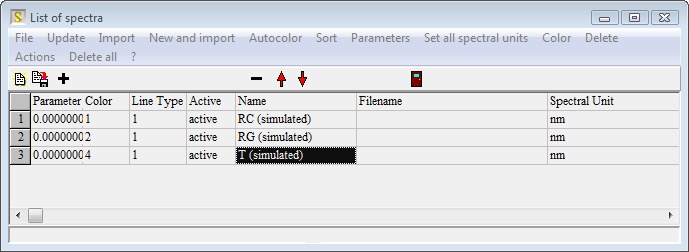
with 3 simulated spectra in one graph:
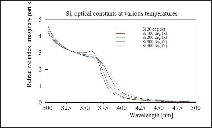
You can also display optical constants in multiple spectra views. In this case you have to refer to the name of the material and specify in addition which quantity you want to display:
o(n) : real part of the refractive index
o(k) : imaginary part of the refractive index
o(real part df) : real part of the dielectric function
o(imaginary part df) : imaginary part of the dielectric function
o(alpha) : intensity absorption coefficient
o(energy loss) : energy loss function
Here is an example:
Drag&Drop creation
You can drag spectra from the list of spectra and drop them on multiple spectra view objects. In this case the view object generates 2 new items in the internal list of spectra, displaying the simulated and measured spectra of the dropped object.
In a similar way you can drag&drop materials to multiple spectra view objects, which tells the object to generate displays of n and k of the dropped material.