Navigation:  Interfaces > Layer stacks

The surface of interface objects can be covered with arbitrary layer stacks. Each layer is 'filled' with optical constants taken from the list of dielectric functions. The top halfspace and the bottom halfspace should have optical constants with small absorption coefficients:

 

 

The window which lets you define the layer stack and some other properties (scatterers, surface tilt angle distribution) looks like this:

 

 

The definition of layer stacks in SPRAY is exactly the same as in SCOUT. Please consult the SCOUT technical manual for details.

 

How it works

If a ray hits an interface with a layer stack SPRAY must decide it the ray gets reflected, transmitted or absorbed.This is done the following way:

Before the ray-tracing for a new spectral point is started the angle dependence of the reflectance and transmittance of the layer stack is computed for both s- and p-polarization. The angle resolution for these calculations is set in the Parameters section.

During the ray-tracing procedure, if a ray hits the surface of an object that is covered with the layer stack, the projection of the ray's polarization onto the direction of s-polarization and p-polarization is determined. With probabilities proportional to these projections the polarization is changed to either pure s- or p-polarization. For the present angle of incidence and polarization, the reflectance and transmittance coefficient is looked up in the previously computed tables. Linear interpolation is used between angles for which the data have been calculated. Based on the values for reflectance and transmittance, it is decided if the ray is reflected, transmitted or absorbed. In the case of reflection the new direction is computed according to the law of reflection. The new direction of a transmitted ray is set applying the law of refraction, taking into account the real part of the index of refraction of top and bottom halfspace.

 

Layer stacks are considered to be infinitely thin with respect to the geometrical dimensions of the objects in the ray-tracing scenery. To be consistent with this assumption, the total thickness of the layer stacks used in a SPRAY simulation must be small enough.

 

Scatterer assignment

All user-defined interfaces can be used as separation between continuum scatterers. Usually the Properties submenu contains a command called Scatterer assignment which opens the following dialog:

 

 

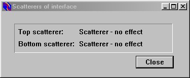
From the list of scatterers you can drag the appropriate scatterers to the top and the bottom halfspace, respectively. The two halfspaces are separated by the interface, of course. The default selection for the scatterers is 'No effect' which means there are no scatterers on both sides of the interface.

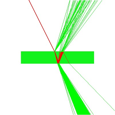
The picture below shows an example: The upper interface (viewed from the side) switches from a non-scattering medium (top) to a light scattering continuum (bottom):

 

 

Introducing surface roughness: Tilt of surface normal

You can introduce surface roughness to the SPRAY model in a simple, statistical way. Instead of explicitly defining a certain surface shape (which is possible with user-defined surface shape objects) you can tilt the surface normal according to a statistical distribution whenever a ray hits the surface. The point where the hit occurs is still determined by the geometric object but the surface normal tilt angle is taken statistically.

Using the menu command Properties|Distribution of surface normal tilt angles you can open a subwindow which is used to define the tilt angle distribution:

 

 

Please note that this window blocks SPRAY until it is closed again: You cannot access other parts of the program as long as this window is open.

The tilt angle distribution is used only if the checkbox 'Active' is checked. It is ignored otherwise.

Depending on the settings of the checkboxes 'Use formula', 'Use lookup table' and 'Use imported data' the angle distribution is computed from a

•user-defined formula: Type in a formula in the edit box to the right of 'Y(X,Y) = ' in the top of the window. In the formula, use the term 'X' to refer to the angle. Click on the menu command Range in order to set the angle range where the formula is going to be evaluated. This can be 0 ... 90 degree or a subrange. Use a large number of points in the range dialog, e.g. 500 or 1000, in order to display the user-defined curve. Finally press Go or Update in order to compute the distribution.

•a lookup table: The distribution is computed using a lookup table. The lookup table is imported from the workbook using the command Workbook|Import lookup table from data columns or Workbook|Import lookup table from data rows. Here is an example of a workbook page with a lookup table:

 

 

Place the cursor into cell B3 and use the command Workbook|Import lookup table from data columns in order to read the table values. Afterwards the points of the lookup table are displayed in the graph:

 

 

Check the option Use lookup table and press Go. Now the distribution is computed using linear interpolation in between the points of the lookup table and constant extrapolation outside the range of the lookup table:

 

 

•a set of imported data points: Use the Import menu command to import the complete angle distribution from a data file. Alternatively, you can import the data using the command Workbook|Import xy (this will read data columns from the workbook, starting at the cursor position). Please read the section 'Technical notes|Import formats' in the SCOUT technical manual for more information on file import data formats.

 

Here is a simple example demonstrating the introduction of surface roughnes using this mechanism of surface normal tilting: A light source illuminates aa glass plate from the upper left. Without surface roughness the ray-tracing looks like this:

 

 

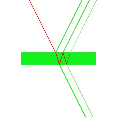
Using the formula exp(-(x/5)^2) the following distribution is created:

 

 

Activating the surface tilt by checking the Active checkbox the ray-tracing changes to this: