Fluorescent scatterers |
  
|
Fluorescent scatterers |
|
Fluorescent scatterers do not only absorb or scatter radiation, but also re-emit radiation at a frequency different form the frequency of the absorbed radiation. In the present implementation the energy of the emitted rays must be lower than the one of the absorbed light. This should be a good approximation in most cases. The energy shift between absorbed and emitted radiation requires some refinement of the SPRAY algorithm to compute spectra which is shortly described below.
The properties of fluorescent scatterers are defined in the following window:

The graph shows four spectra:
•The blue curve gives the probability / distance (in cm) for absorption without further re-emission.
•The red spectrum is the probability / distance for isotropic scattering without energy shift (sometimes called 'Elastic scattering').
•The solid green line shows the probability / distance for absorption and subsequent re-emission at lower energy (fluorescence).
•The dashed green line gives the spectral composition of the re-emitted low frequency radiation.
At present, all four probability curves are imported from text files (extension *.ifd) which have the following structure:
10000 0.0002849304889 0.0001424652444 5.698609778E-005 1.388794386E-011
10100 0.0003091027739 0.000154551387 6.182055478E-005 3.737571328E-011
10200 0.0003351888926 0.0001675944463 6.703777852E-005 9.859505576E-011
10300 0.0003633281703 0 .0001816640852 7.266563406E-005 2.54938188E-010
10400 0.0003936690407 0.0001968345203 7.873380813E-005 6.461431773E-010
10500 0004263695576 0.0002131847788 8.527391152E-005 1.605228055E-009
10600 0.0004615979303 0.0002307989652 9.231958606E-005 3.908938434E-009
10700 0.0004995330806 0.0002497665403 9.990661611E-005 9.330287575E-009
10800 0.0005403652241 0.000270182612 0.0001080730448 2.182957795E-008
10900 0.0005842964753 0.0002921482376 .0001168592951 5.006218021E-008
11000 0.0006315414766 0.0003157707383 0.0001263082953 1.125351747E-007
11100 0.0006823280528 0.0003411640264 0.0001364656106 2.479596018E-007
.
.
.
The first column is the spectral position. It must be specified using wavenumbers (inverse wavelength, the unit is 1/cm). The second column is the probability / distance (in cm) for absorption without further re-emission (the blue curve above), followed by the probability for isotropic scattering without energy change (red curve) and the absorption probability with energy shift (green solid line). Finally, the last column gives the frequency distribution of the re-emitted fluorescent radiation (which is isotropic concerning the direction distribution).
The input data for fluorescent scatterer objects can conveniently be created using the Data Factory utility (which is delivered with SPRAY) and the built-in workbook. Once you have computed and copied all required data columns into the right sequence you can export the workbook data using the text file format 'Tabbed text'.
The SPRAY algorithm to do ray-tracing simulations has been extended in order to include the energy shifts caused by fluorescent scatterers. SPRAY always does the loop through all spectral points starting at the highest energy. If you use eV, 1/cm or THz, it will start with the highest value. If wavelengths (nm or microns) are selected, SPRAY will start with the lowest value.
During the simulation, SPRAY collects all rays which are absorbed by a fluorescent scatterer and for which re-emission occurs. The rays are added to a queue at the energy selected for re-emission. After all rays emitted by the light source are processed for a spectral point, SPRAY checks if there are 'fluorescent' rays in the queue to be re-started at this frequency. Of course, the rays are started where there were absorbed previously. This way the algorithm includes multiple absorption-emission cycles. However, only energy shifts towards lower energies are possible at the moment.
A simple example demonstrates the use of fluorescent scatterers. A circular light source illuminates a cylinder filled with the scatterers. The probabilities shown in the graph above are used.
Two detectors register radiation: One collects rays moving in the direction of the radiation emitted by light source (mainly un-absorbed and un-scattered rays are found here), one 'sees' rays scattered to the side (elastically scattered radiation as well as fluorescence light).
The 'forward detector' spectrum is this:

Below 600 nm the spectrum is dominated by the large absorption/scattering losses whereas in the infrared region almost all rays move through the cylinder without modification. Around 680 nm the sum of re-emitted rays from higher energies and unscattered and elastically scattered rays is larger than the number of rays emitted by the light source in this spectral range. Hence the detector signal is larger than 1 which may occur in the case of fluorescence.
The detector recording the radiation scattered sideways has the following spectrum:
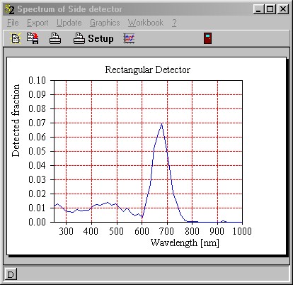
Here we see the superposition of elastically scattered light (the broad distribution below 800 nm) and the sharper peak of fluorescence light around 680 nm.