Navigation:  Quick start: Getting around in SCOUT > Building a simple optical model

We will now setup the optical model the following way:

 

•Take the optical constants of glass and silver from the database

•Compose the layer stack

•Setup the reflectance spectrum

•Select the fit parameters

 

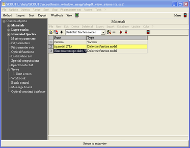
All required actions are done in the treeview level. Right-click the treeview branch 'Optical constant database' and select in the list of database materials the one called 'Ag model (TL)':

 

 

With the left mouse button, drag&drop it to the treeview branch called Materials. Repeat this step for the material called 'Glass (microscope slide), Vis'. Now right-click the treeview branch Materials in order to open the current list of materials. It should look like this now:

 

 

With these materials in our configuration, we are now ready to define the layer stack. Open the treeview branch Layer stacks. This list may contain several layer stacks. In this simple example, we need a single stack only. Right-click the treeview item 'Layer stack'  which should look like this at the moment:

 

 

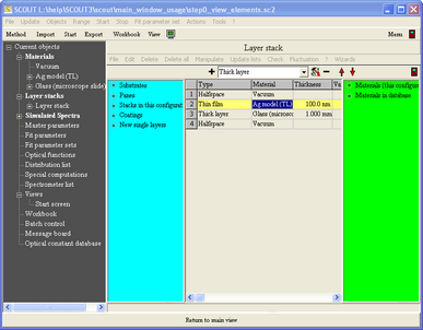
Select the bottom halfspace in the layer stack and use the + button in order to create a layer of type 'Thin film'. This will be used to represent the silver layer. Afterwards, select the new layer type 'Thick layer' and generate an object of this type which we will use for the glass substrate. Using the red arrow buttons, bring the objects into the following order:

 

 

We will now assign materials to the individual layers. Open the Materials branch in the treeview. Drag the treeview item 'Ag model (TL)' to layer #2 in the stack and drop it there. Repeat this drag&drop for the glass material. The layer stack should look like this after these actions:

 

 

Having defined all required materials and the layer stack, we can now compute the reflectance spectrum of the layer stack. The experimental data that we are going to load have been measured in the spectral range 200 ... 1100 nm. Hence it makes sense to compute the optical model in this range. Since the loaded materials are models for optical constants (indicated by their type 'Dielectric function model') it is useful to compute the material models as well as the spectrum in the same wavelength range 200 ... 1100 nm. We can achieve this by using the global Range command in the main menu of SCOUT. A spectral range dialog appears and you should do the following settings:

 

 

The reflectance spectrum must be defined in the list of simulated spectra. Open the corresponding treeview branch which contains an object already (if not in your situation, please select the new object type 'R, T, ATR' in the dropdown box and generate an object of this type):

 

 

In order to have a closer look at the spectrum, open the tree branch 'Simulated spectra' by clicking at the + symbol and right-click the object 'R':

 

 

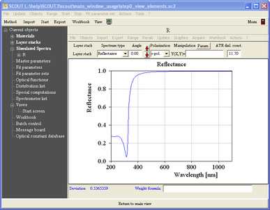
This shows already the wanted reflectance spectrum (the angle of 0° is a good approximation in the present case). We only have to adjust the axis settings for the graph which we can do using the local menu item 'Graphics|Edit plotparameters'. Please use the following settings in the graphics parameters dialog:

 

 

After pressing OK the graph is updated and looks like this now:

 

 

The optical model is ready now. The simulated reflectance can be compared to measured data. Use the local menu command Import|from file to load experimental spectra from data files. The spectra we are using here are distributed with SCOUT tutorial 1. Open the file ag_20.std from the SCOUT tutorial 1 subfolder using the file type 'SCOUT standard format' as indicated in the following screenshot:

 

 

Make sure that you select the spectral unit nm in the following dialog which shows the spectral range covered by the data found in the file:

 

 

After pressing OK the spectrum window looks like this now:

 

 

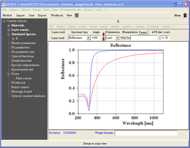
The red curve shows the loaded experimental data whereas the blue one represents the current model.

 

Obviously there is a significant disagreement between model and measurement which is a good reason to modify the model. The thickness of the silver layer is the parameter of the model which needs to be adapted in order to improve the agreement. We have to declare the silver thickness to be a fit parameter in order to do an automatic parameter adjustment (fit). Right-click the treeview branch Fit parameters:

 

 

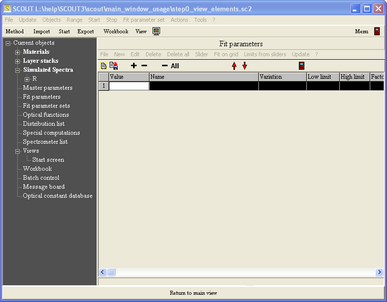
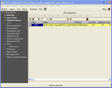
Note that the list of fit parameters has no dropdown box in order to specify object types. There is only one type of objects in this list. Press the + button and you will get a dialog which displays all current model parameters. Select the silver thickness as shown below (while holding the ctrl-key down, you can select and de-select multiple items in this dialog by mouse-clicks):

 

 

With this selection, leave the dialog pressing OK. The list of fit parameters is now the following:

 

 

The current problem is quite simple, and we can hope that the automatic fit routine of SCOUT can find the best value for the thickness without further help. Press Start in the toolbar to launch the fit routine (this button becomes a red Stop button while the fit is running). After a very short time the fit finishes and the red Stop button becomes a black Start button again.

Right-click the spectrum object R in the treeview and see the following fit result:

 

 

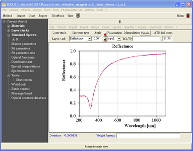
We have now an optical model matching the experimental results. If we want to do parameter fits for several experimental input spectra it might be useful to build a simple user-interface which offers the required actions in the main view. This will be done in the next section.