About SCOUT |
  
|
About SCOUT |
|
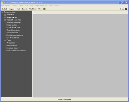
SCOUT is a Windows NT/2000/XP/Vista software for the analysis of optical spectra by computer simulation. At program start the main window opens which may look like this:

The main window has 2 levels. When the program starts, you see the so-called 'main view level' which consists of the
•menu, from which all parts of the program can be reached
•the toolbar (below the menu), featuring selected commands for easy access
•the drawing area (the blue part in the example above) showing the main view (text, spectra, parameter values or illustrative graphs, see user-defined views)
•and the status bar at the bottom (including information and some control elements for the displayed graphs)
Pressing F7 the main window switches to the 'treeview level' which looks like this:
On the left side you see a treeview of all objects in the current SCOUT configuration. With a right click on an object in the tree you can open it - most objects will display their controls or graphs in the right gray section. Whereas some objects will display only a few items or even nothing, others will show a graph, buttons and an object menu. Here is the example of an opened spectrum window:
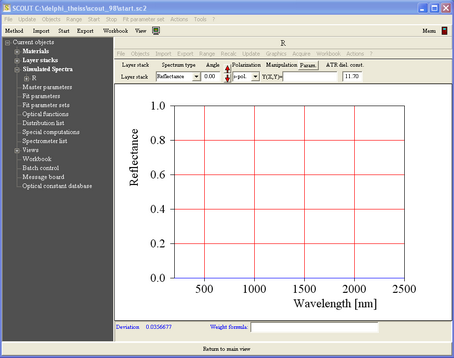
Pressing F7 again switches SCOUT back to the main view level. Alternatively, you can press the large 'Return to main view' button at the bottom of the window.
See the chapter 'Quick start: Getting around in SCOUT' for a deeper user interface description.
Working with pre-defined configurations, using the main window only
If you belong to the lucky people that can work with pre-defined SCOUT configurations, and you don't have to develop optical models of your own, it might be sufficient for you to only read the section about using the main window. However, if you are eager to know how the program works, you can read the other parts of this manual as well. This will certainly help to improve your SCOUT skills.
Required steps for developing optical models
Advanced spectrum simulation is not easy. Setting up realistic optical models, you have to define a large number of parameters which reflect the complexity of the problem. Concerning its structure, SCOUT tries to be as close to the physical problem as possible and groups the many parameters of spectrum simulation according to the scheme described below.
1. Define the optical constants of all relevant materials
All optical constant definitions are done in the so-called material list which you can access from the main window by pressing F7. Materials are managed in the first branch of the object tree called Materials. Here you can define objects representing fixed optical constants (imported from files) or optical constant models that give you flexibility if you want to adjust optical constants to fit experimental data.
Optical constant models are composed of susceptibility terms which are managed in susceptibility lists. At present you can use the following types:
Drude model for free carriers
Extended Drude model for free carriers with frequency dependent damping
extended oscillator model suggested by Brendel
extended oscillator model suggested by Kim
oscillator model suggested by Gervais
OJL interband transition model
Campi-Coriasso interband transition model
Tauc-Lorentz interband transition model
user-defined expressions for optical constants
Both fixed optical constants and models can be imported easily from the built in database of optical constants.
For the description of heterogeneous materials (two-phase composites) you may want to mix optical constants. This can be done in SCOUT using various effective medium concepts for inhomogeneous materials. Besides the classical Maxwell Garnett and Bruggeman approaches we offer the Looyenga formula and the general Bergman representation which is certainly the most advanced concept.
2. Define the structure of the layer stacks
The tree branch Layer stacks shows the list of layer stacks. In most cases you will investigate one layer stack only, but SCOUT lets you work with several stacks if you want to (or have to).
Each layer stack may consist of an unlimited number of layers which are again managed in lists, called layer stack. For simple layers you can select coherent or incoherent superposition of partial waves. Several types reflect a certain choice: A 'Thin film' is always handled with coherent superposition whereas a layer of type 'Thick layer' is treated with incoherent superposition. For cases in between full coherent or incoherent superposition we have implemented an efficient averaging algorithm for lateral layer thickness inhomogeneities. You can define optical superlattices, corrections for scattering losses at rough interfaces and gradually changing optical properties. Anisotropic layers (with heavy restrictions at the moment) may also occur in the stack.
3. Define which type of spectra are to be simulated and compared to experiments
After the definiton of all optical constants and layer stacks you have to tell SCOUT which spectra it should simulate and compare to experimental data. These spectra are collected in the spectra list which is the Simulated spectra branch in the treeview. The following types of spectra can be used at present:
•ATR
•Layer Mix (computes the average spectrum of a patterned sample)
•Layer absorption (computes the absorbed fraction of incident light intensity in a certain layer in a stack)
•Charge carrier generation (computes the number of photon-generated charge carriers in a layer)
4. Select the fit parameters
The treeview branch Fit parameters holds the list of fit parameters. These are the parameters of the model that are to be adjusted in order to reach optimal agreement between simulation and measurements. Besides fitting to experimental data, you can also select a model parameter as fit parameter if you want to compute its value by a user-defined function (which may contain master parameters, optical function values or the time).
5. Fit of the model (manual, visual, automatic)
SCOUT lets you fit model parameters manually (type in new values) or visually, i.e. by mouse-driven sliders. With the 'fit on a grid' feature you can automatically scan a certain parameter range for the best starting value for the final completely automatic optimization.
Using sequences of fit parameter sets (available in the treeview branch Fit parameter sets) you can develop efficient optimization strategies which enable SCOUT to adjust many fit parameters completely automatic.
In cases for which completely automatic parameter fitting is possible you can process a whole series of input spectra in a batch operation. SCOUT will import the spectra, do the fit, and store the obtained results in appropriate tables.
Enhancing your SCOUT work
Customizing SCOUT for routine spectroscopy using Views and the toolbar
Once you have developed a convincing optical model that reproduces your measurements in a high quality you may want to make that solution accessible to other people which are probably less experienced. In this case, you can hide all the complexity of the model and show in the main window only the information relevant to the final result. Using Views and the flexible toolbar you can achieve this goal and create nice and simple user interfaces.
Inspecting the influence of model parameters on optical spectra
Some automized actions help you to find out how model parameters affect optical spectra. You can vary one selected parameter on a set of equidistant values (in a user-defined range) using the Parameter variation action. SCOUT will compute all defined spectra for the set of values, and you can generate quite useful plots visualizing the parameter influence.
In order to check how production tolerances influence the optical properties of your multilayer stack, you can compute the spectral variations for the case that some model parameters fluctuate randomly in user-defined intervals (Parameter fluctuation action).
Working with databases
You can work with SCOUT very efficiently making use of databases. A SCOUT database contains materials with pre-defined optical constants and pre-defined layer stacks. If you save your favourite substrates and materials to your personal database these objects can be used to quickly build SCOUT configurations from scratch.
You can also benefit from the large collection of optical constants which is stored in the SCOUT database.
Programming SCOUT by OLE automation
You can control the actions of SCOUT from external programs by OLE automation. Create automated reports and batch operations with the Windows Scripting Host (WSH), MS Word, MS Excel, LabView or any other OLE automation controller. Using OLE automation you can even hide SCOUT completely, feed it with spectra and have it doing the analysis in the background while your data acquisition hardware collects already the next set of spectra .
To get a quick start into the details of spectrum simulation you should follow the introductory SCOUT tutorials (which are distributed with SCOUT and also available on our homepage www.mtheiss.com in the support section).
You can also have a look at the following documents which are distributed as PDF documents on the SCOUT CD (folder docs). You can also download these documents from our homepage using the link http://www.mtheiss.com/?Support:Downloads:Things_to_read:
•Analyzing optical spectra by computer simulation - from basics to batch mode (a PDF-document about spectrum simulation, summarizing the background and typical applications of this technique)
•Developing optical production control methods for SCOUT (a PDF-document about developing SCOUT methods. Good to read if you are looking for a thin film production control solution - even if you are not developing the method yourself but let us do the work)